Using spatialDWLS from Giotto

Giotto calls spatialDWLS through runDWLSDeconv(), so a Giotto user never touches the matrices directly: the expression, clusters and result all stay in the Giotto object. This article shows that workflow on the small Visium dataset that ships with GiottoData. For the same method on plain matrices, see Get started.

The outputs on this page were computed locally and saved, because building them needs Giotto, GiottoData and a Giotto environment. The script that produced them is dev/render-giotto-article.R.

Setup

spatialDWLS is a suggested package of Giotto, so install both:

remotes::install_github("drieslab/spatialDWLS")
# and Giotto: https://giottosuite.com/articles/installation.html

library(Giotto)

g <- GiottoData::loadGiottoMini("visium")

The mini object is a small mouse brain Visium section that has already been normalised and clustered (leiden_clus).

1. A signature matrix

spatialDWLS needs the mean expression of each cell type over a set of signature genes. In a real analysis that comes from a single-cell reference of the same tissue, for example with makeSignMatrixDWLSfromMatrix() on the reference’s normalised expression and its cell type labels.

GiottoData has no matching single-cell reference, so for this demonstration the “cell types” are the Visium clusters themselves and the signature genes are their top markers. That is enough to show the workflow; it is not how to get biologically meaningful cell types.

markers <- findMarkers_one_vs_all(g, method = "scran",
                                  cluster_column = "leiden_clus",
                                  min_feats = 20)
sign_gene <- unique(markers[, head(feats, 20), by = "cluster"]$V1)

meta <- pDataDT(g)
sign_matrix <- makeSignMatrixDWLS(g,
  sign_gene = sign_gene,
  cell_type_vector = paste0("type_", meta$leiden_clus)
)
dim(sign_matrix)

#> [1] 123   7

2. Deconvolve

g <- runDWLSDeconv(g,
  sign_matrix = sign_matrix,
  cluster_column = "leiden_clus",
  n_cell = 10
)

The proportions are stored in the object as a spatial enrichment named "DWLS", one row per spot:

getSpatialEnrichment(g, name = "DWLS", output = "data.table")

#>               cell_ID type_1 type_2 type_3 type_4 type_5    type_6    type_7
#>                <char>  <num>  <num>  <num>  <num>  <num>     <num>     <num>
#> 1: AAAGGGATGTAGCAAG-1      0      0      0      0      0 0.5209807 0.4790193
#> 2: AAATGGCATGTCTTGT-1      1      0      0      0      0 0.0000000 0.0000000
#> 3: AAATGGTCAATGTGCC-1      0      0      1      0      0 0.0000000 0.0000000
#> 4: AAATTAACGGGTAGCT-1      0      0      1      0      0 0.0000000 0.0000000

runDWLSDeconv() takes the same settings as spatialDWLS::dwls():

• n_cell: expected cells per spot. A cell type is kept for a spot in the second round only when its first-round share is at least 1 / n_cell.
• cutoff: the enrichment score a cell type must reach in a cluster to be considered there.
• BPPARAM: run the per-spot solves in parallel, e.g. BPPARAM = BiocParallel::MulticoreParam(8). Without it, Giotto’s session default (GiottoUtils::giotto_bpparam()) is used.
• na_as_zero: spots with no signal on the signature genes are NA by default.

3. Plot

spatDeconvPlot() draws each spot as a pie of its cell type proportions:

spatDeconvPlot(g, deconv_name = "DWLS", pie_scale = 0.4)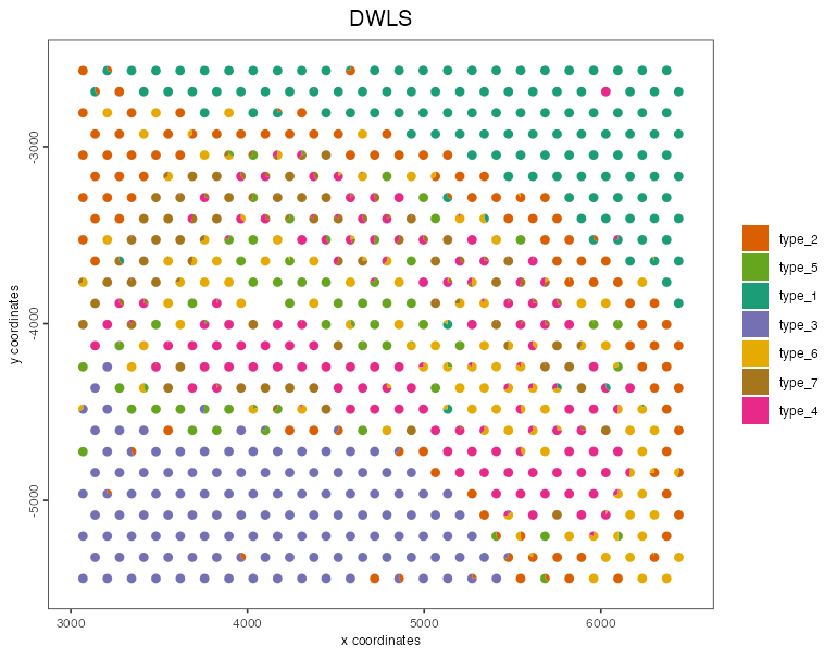

The proportions are ordinary columns, so anything else is a short step away, e.g. colouring spots by their dominant cell type:

dwls <- getSpatialEnrichment(g, name = "DWLS", output = "data.table")
type_cols <- setdiff(names(dwls), "cell_ID")
dominant <- type_cols[max.col(as.matrix(dwls[, type_cols, with = FALSE]))]

g <- addCellMetadata(g,
  new_metadata = data.frame(cell_ID = dwls$cell_ID, dominant_type = dominant),
  by_column = TRUE, column_cell_ID = "cell_ID"
)
spatPlot2D(g, cell_color = "dominant_type", point_size = 2.5)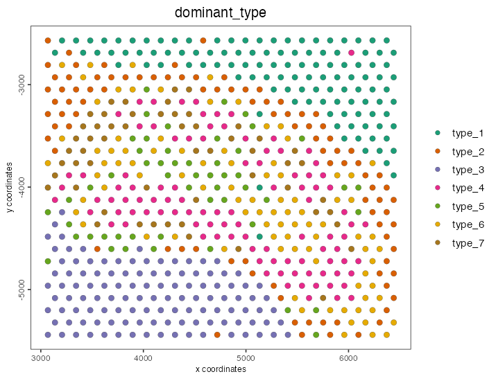

Disk-backed objects

A Giotto object whose expression is held on disk by GiottoDisk goes through the same runDWLSDeconv() call. GiottoDisk reads the signature genes one window of spots at a time and hands them to spatialDWLS::dwls_stream(), so the result is the same while the expression never has to fit in memory.