Get started with spatialDWLS

This example uses nothing but matrices: no Giotto, no Seurat, no SpatialExperiment. If your data already lives in a Giotto object, see Using spatialDWLS from Giotto instead.

spatialDWLS needs three things:

1. Spot expression: log-normalised, features x spots.
2. A reference: mean expression of each cell type over a set of signature features, built from single-cell data.
3. A cluster per spot: spots are grouped to decide which cell types are plausible where. Any clustering of the spots works (e.g. Leiden on the expression).

library(spatialDWLS)
library(Matrix)

Simulate a small dataset with known answers

To be able to check the result, we simulate spots whose true composition is known. Eight cell types each get 40 marker genes; each spot holds 2 to 10 cells drawn from one of six tissue niches; the niche is the spot’s cluster.

set.seed(1)
n_genes <- 1500; n_types <- 8; n_spots <- 400
types <- paste0("type", seq_len(n_types))

# expression profile of each cell type
profile <- matrix(rlnorm(n_genes), n_genes, n_types,
                  dimnames = list(paste0("g", seq_len(n_genes)), types))
markers <- split(sample(n_genes, 40 * n_types), rep(types, each = 40))
for (ct in types) {
  profile[markers[[ct]], ct] <- profile[markers[[ct]], ct] * runif(40, 4, 10)
}
profile <- sweep(profile, 2, colSums(profile), "/") * 5000

normalise <- function(counts) {
  counts <- Matrix(counts, sparse = TRUE)
  t(t(counts) / pmax(colSums(counts), 1)) * 1e4
}

# a single-cell reference: 60 cells per type
ref_type <- rep(types, each = 60)
ref <- matrix(rpois(n_genes * length(ref_type), profile[, ref_type] * 0.3),
              n_genes, dimnames = list(rownames(profile), NULL))

# spots: each niche favours a few cell types
niche_mix <- t(replicate(6, { p <- rgamma(n_types, 0.3); p / sum(p) }))
niche <- sample(6, n_spots, replace = TRUE)
cells <- sample(2:10, n_spots, replace = TRUE)
composition <- sapply(seq_len(n_spots), function(s) {
  rmultinom(1, cells[s], niche_mix[niche[s], ])
})
spot_counts <- matrix(rpois(n_genes * n_spots, profile %*% composition * 0.5),
                      n_genes, dimnames = list(rownames(profile),
                                               paste0("spot", seq_len(n_spots))))
truth <- sweep(composition, 2, cells, "/")
dimnames(truth) <- list(types, colnames(spot_counts))

1. Build the reference

dwls_signature() averages each cell type over the signature features. Pass the reference on the normalised, not logged scale: that is the scale the spots are solved on.

signature <- dwls_signature(normalise(ref),
                            sign_gene = rownames(profile)[unlist(markers)],
                            cell_type = ref_type)
dim(signature)
#> [1] 320   8
round(signature[1:4, 1:4], 1)
#>     type1 type2 type3 type4
#> g12   4.7   4.6  28.5   5.2
#> g15  10.7   9.3  10.4  11.5
#> g17   2.8   3.5  15.2   3.4
#> g27   2.7   1.7   2.7  18.3

2. Deconvolve

The spots go in log-normalised, as most pipelines store them. Sparse input stays sparse.

spot_expr <- normalise(spot_counts)
spot_expr@x <- log2(spot_expr@x + 1)
clusters <- paste0("niche", niche)

prop <- dwls(spot_expr, signature, clusters, n_cell = 10)
dim(prop)
#> [1]   8 400
round(prop[, 1:5], 2)
#>       spot1 spot2 spot3 spot4 spot5
#> type1  0.00  0.34  0.65  0.00  0.00
#> type2  0.00  0.00  0.14  0.00  0.00
#> type3  0.65  0.00  0.00  0.51  0.00
#> type4  0.00  0.32  0.00  0.00  0.00
#> type5  0.35  0.34  0.22  0.00  0.13
#> type6  0.00  0.00  0.00  0.00  0.87
#> type7  0.00  0.00  0.00  0.10  0.00
#> type8  0.00  0.00  0.00  0.39  0.00

prop holds one column per spot and one row per cell type. Each spot sums to one:

summary(colSums(prop))
#>    Min. 1st Qu.  Median    Mean 3rd Qu.    Max. 
#>       1       1       1       1       1       1

n_cell is the number of cells you expect in a spot. In the second round a cell type is only kept for a spot when its first-round share is at least 1 / n_cell, so it sets how small a contribution is still believed.

3. Check against the truth

plot(truth, prop[rownames(truth), ], pch = 16, cex = 0.5,
     col = adjustcolor("steelblue", 0.4),
     xlab = "true proportion", ylab = "spatialDWLS estimate")
abline(0, 1, lty = 2)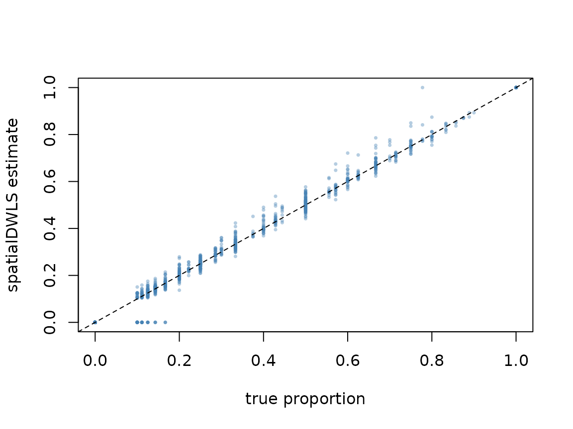

sqrt(mean((prop[rownames(truth), ] - truth)^2))  # RMSE
#> [1] 0.01920764

Larger data

In parallel. Pass any BiocParallel param. The result is identical to the serial run.

prop <- dwls(spot_expr, signature, clusters, n_cell = 10,
             BPPARAM = BiocParallel::MulticoreParam(8))

More spots than memory. dwls_stream() asks for the expression one window of spots at a time, through a function you supply, and only for the signature features. The windows here are just column blocks of the matrix, but read_window could equally read from disk.

windows <- split(colnames(spot_expr), ceiling(seq_len(n_spots) / 100))
read_window <- function(i, features) spot_expr[features, windows[[i]]]

prop_streamed <- dwls_stream(
  read_window = read_window,
  n_windows = length(windows),
  feat_ids = rownames(spot_expr),
  clusters = setNames(clusters, colnames(spot_expr)),
  sign_matrix = signature,
  n_cell = 10
)
all.equal(prop_streamed, prop)
#> [1] TRUE

Reference

Dong R, Yuan GC (2021). SpatialDWLS: accurate deconvolution of spatial transcriptomic data. Genome Biology 22, 145. https://doi.org/10.1186/s13059-021-02362-7