Visualize gene expression according to dimension reduction coordinates
Usage
dimFeatPlot2D(
  gobject,
  spat_unit = NULL,
  feat_type = NULL,
  expression_values = c("normalized", "scaled", "custom"),
  feats = NULL,
  order = TRUE,
  group_by = NULL,
  group_by_subset = NULL,
  dim_reduction_to_use = "umap",
  dim_reduction_name = NULL,
  dim1_to_use = 1,
  dim2_to_use = 2,
  show_NN_network = FALSE,
  nn_network_to_use = "sNN",
  network_name = "sNN.pca",
  network_color = "lightgray",
  edge_alpha = NULL,
  scale_alpha_with_expression = FALSE,
  point_shape = c("border", "no_border"),
  point_size = 1,
  point_alpha = 1,
  cell_color_gradient = NULL,
  gradient_midpoint = NULL,
  gradient_style = c("divergent", "sequential"),
  gradient_limits = NULL,
  point_border_col = "black",
  point_border_stroke = 0.1,
  show_legend = TRUE,
  legend_text = 10,
  background_color = "white",
  axis_text = 8,
  axis_title = 8,
  cow_n_col = NULL,
  cow_rel_h = 1,
  cow_rel_w = 1,
  cow_align = "h",
  show_plot = NULL,
  return_plot = NULL,
  save_plot = NULL,
  save_param = list(),
  default_save_name = "dimFeatPlot2D"
)
Arguments
- gobject
giotto object
- spat_unit
spatial unit (e.g. "cell")
- feat_type
feature type (e.g. "rna", "dna", "protein")
- expression_values
gene expression values to use
- feats
features to show
- order
order points according to feature expression
- group_by
character. Create multiple plots based on cell annotation column
- group_by_subset
character. subset the group_by factor column
- dim_reduction_to_use
character. dimension reduction to use
- dim_reduction_name
character. dimension reduction name
- dim1_to_use
numeric. dimension to use on x-axis
- dim2_to_use
numeric. dimension to use on y-axis
- show_NN_network
logical. Show underlying NN network
- nn_network_to_use
character. type of NN network to use (kNN vs sNN)
- network_name
character. name of NN network to use, if show_NN_network = TRUE
- network_color
color of NN network
- edge_alpha
column to use for alpha of the edges
- scale_alpha_with_expression
scale expression with ggplot alpha parameter
- point_shape
point with border or not (border or no_border)
- point_size
size of point (cell)
- point_alpha
transparency of points
- cell_color_gradient
character. continuous colors to use. palette to use or vector of colors to use (minimum of 2).
- gradient_midpoint
numeric. midpoint for color gradient
- gradient_style
either 'divergent' (midpoint is used in color scaling) or 'sequential' (scaled based on data range)
- gradient_limits
numeric vector with lower and upper limits
- point_border_col
color of border around points
- point_border_stroke
stroke size of border around points
- show_legend
logical. show legend
- legend_text
size of legend text
- background_color
color of plot background
- axis_text
size of axis text
- axis_title
size of axis title
- cow_n_col
cowplot param: how many columns
- cow_rel_h
cowplot param: relative heights of rows (e.g. c(1,2))
- cow_rel_w
cowplot param: relative widths of columns (e.g. c(1,2))
- cow_align
cowplot param: how to align
- show_plot
logical. show plot
- return_plot
logical. return ggplot object
- save_plot
logical. save the plot
- save_param
list of saving parameters, see
showSaveParameters- default_save_name
default save name for saving, don't change, change save_name in save_param
Examples
g <- GiottoData::loadGiottoMini("visium", verbose = FALSE)
dimFeatPlot2D(g, feats = c("Gna12", "Ccnd2", "Btbd17"))
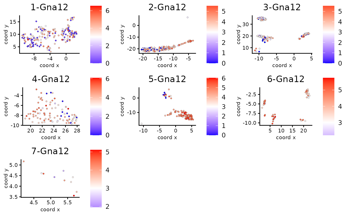
 # with group_by
dimFeatPlot2D(g,
feats = c("Gna12"),
group_by = "leiden_clus",
gradient_midpoint = 3 # setting a specific midpoint can be helpful
)
# with group_by
dimFeatPlot2D(g,
feats = c("Gna12"),
group_by = "leiden_clus",
gradient_midpoint = 3 # setting a specific midpoint can be helpful
)
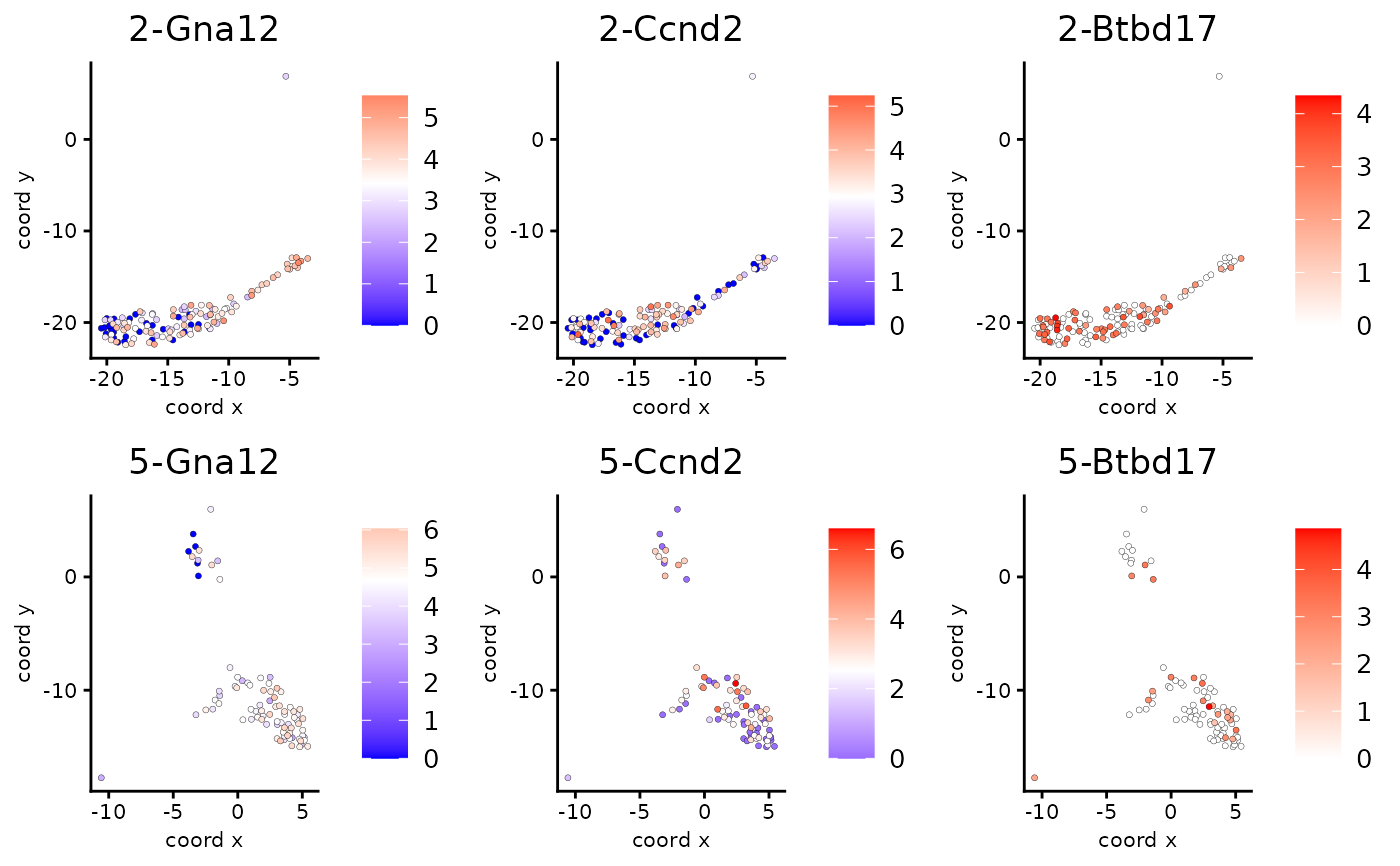
 # with group_by and group_by_subset
dimFeatPlot2D(g,
feats = c("Gna12", "Ccnd2", "Btbd17"),
group_by = "leiden_clus",
group_by_subset = c(2, 5)
)
# with group_by and group_by_subset
dimFeatPlot2D(g,
feats = c("Gna12", "Ccnd2", "Btbd17"),
group_by = "leiden_clus",
group_by_subset = c(2, 5)
)