6 Creating a Giotto object
Jiaji George Chen
August 5th 2024
6.1 Overview
The minimal amount of raw data needed to put together a fully functional giotto object are either of the following:
- spatial coordinates (centroids) and expression matrix information
- spatial feature information (points or image intensity values) and spatial annotations to aggregate that feature information with (polygons/mask).
You can either use the create* style functions introduced in the previous session and build up the object piecewise or you can use the giotto object constructor functions createGiottoObject() and createGiottoObjectSubcellular()
6.2 GiottoData modular package
We can showcase the construction of objects by pulling some raw data from the GiottoData package. A dataset was loaded from here earlier in the previous section, but to formally introduce it, this package contains mini datasets and also download links to other publicly available datasets. It helps with prototyping and development and also making reproducible examples.
The mini examples from popular platform datasets can also help give an understanding of what their data is like and how Giotto represents them.
6.3 From matrix + locations
For this, we will load some visium expression information and spatial locations.
library(Giotto)

# function to get a filepath from GiottoData
mini_vis_raw <- function(x) {
  system.file(
    package = "GiottoData",
    file.path("Mini_datasets", "Visium", "Raw", x)
  )
}

mini_vis_expr <- mini_vis_raw("visium_DG_expr.txt.gz") |>
  data.table::fread() |>
  GiottoUtils::dt_to_matrix()

mini_vis_expr[seq(5), seq(5)]
5 x 5 sparse Matrix of class "dgCMatrix"
AAAGGGATGTAGCAAG-1 AAATGGCATGTCTTGT-1 AAATGGTCAATGTGCC-1 AAATTAACGGGTAGCT-1 AACAACTGGTAGTTGC-1
Gna12 1 2 1 1 9
Ccnd2 . 1 1 . .
Btbd17 . 1 1 1 .
Sox9 . . . . .
Sez6 . 1 4 3 .V1 V2
<int> <int>
1: 5477 -4125
2: 5959 -2808
3: 4720 -5202
4: 5202 -5322
5: 4101 -4604
6: 5821 -3047With these two pieces of data, we can make a fully working giotto object. The spatial locations are missing cell_ID names, but they will be detected from the expression information.
mini_vis <- createGiottoObject(
  expression = mini_vis_expr,
  spatial_locs = mini_vis_slocs
)

instructions(mini_vis, "return_plot") <- FALSE
# set return_plot = FALSE otherwise we will get duplicate outputs in code chunks
For a simple example plot:
spatFeatPlot2D(mini_vis,
               feats = c("Gna12", "Gfap"),
               expression_values = "raw",
               point_size = 2.5,
               gradient_style = "sequential",
               background_color = "black"
)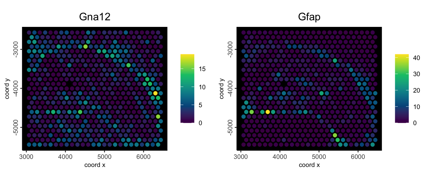
Figure 6.1: Example spatial feature plot to show functioning object
6.4 From subcellular raw data (transcripts or images) + polygons
You can also make giotto objects starting from raw spatial feature information and annotations that give them spatial context.
# function to get a filepath from GiottoData
mini_viz_raw <- function(x) {
  system.file(
    package = "GiottoData",
    file.path("Mini_datasets", "Vizgen", "Raw", x)
  )
}

mini_viz_dt <- mini_viz_raw(file.path("cell_boundaries", "z0_polygons.gz")) |>
  data.table::fread()

mini_viz_poly <- createGiottoPolygon(mini_viz_dt)

force(mini_viz_poly)
An object of class giottoPolygon
spat_unit : "cell"
Spatial Information:
class : SpatVector
geometry : polygons
dimensions : 498, 1 (geometries, attributes)
extent : 6399.244, 6903.243, -5152.39, -4694.868 (xmin, xmax, ymin, ymax)
coord. ref. :
names : poly_ID
type : <chr>
values : 40951783403982682273285375368232495429
240649020551054330404932383065726870513
274176126496863898679934791272921588227
centroids : NULL
overlaps : NULL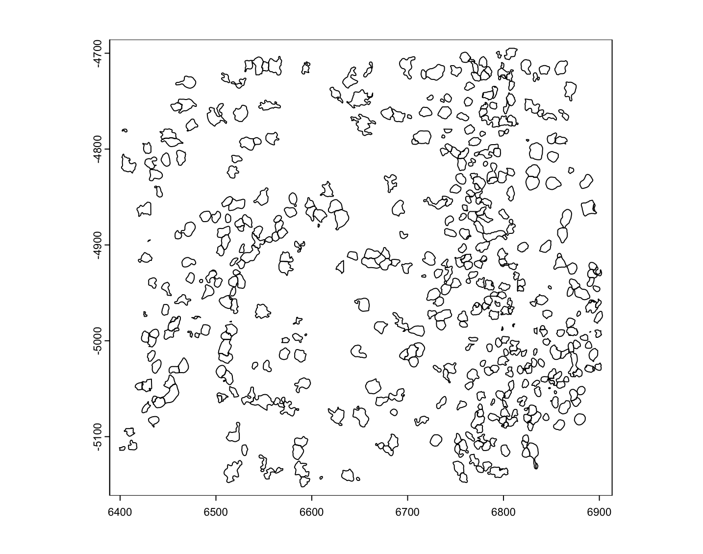
Figure 6.2: Example MERSCOPE polygons loaded form vertex info
mini_viz_tx <- mini_viz_raw("vizgen_transcripts.gz") |>
  data.table::fread()

mini_viz_tx[, global_y := -global_y] # flip values to match polys

viz_gpoints <- createGiottoPoints(mini_viz_tx)

force(viz_gpoints)
An object of class giottoPoints
feat_type : "rna"
Feature Information:
class : SpatVector
geometry : points
dimensions : 80343, 3 (geometries, attributes)
extent : 6400.037, 6900.032, 4699.979, 5149.983 (xmin, xmax, ymin, ymax)
coord. ref. :
names : feat_ID global_z feat_ID_uniq
type : <chr> <int> <int>
values : Mlc1 0 1
Gprc5b 0 2
Gfap 0 3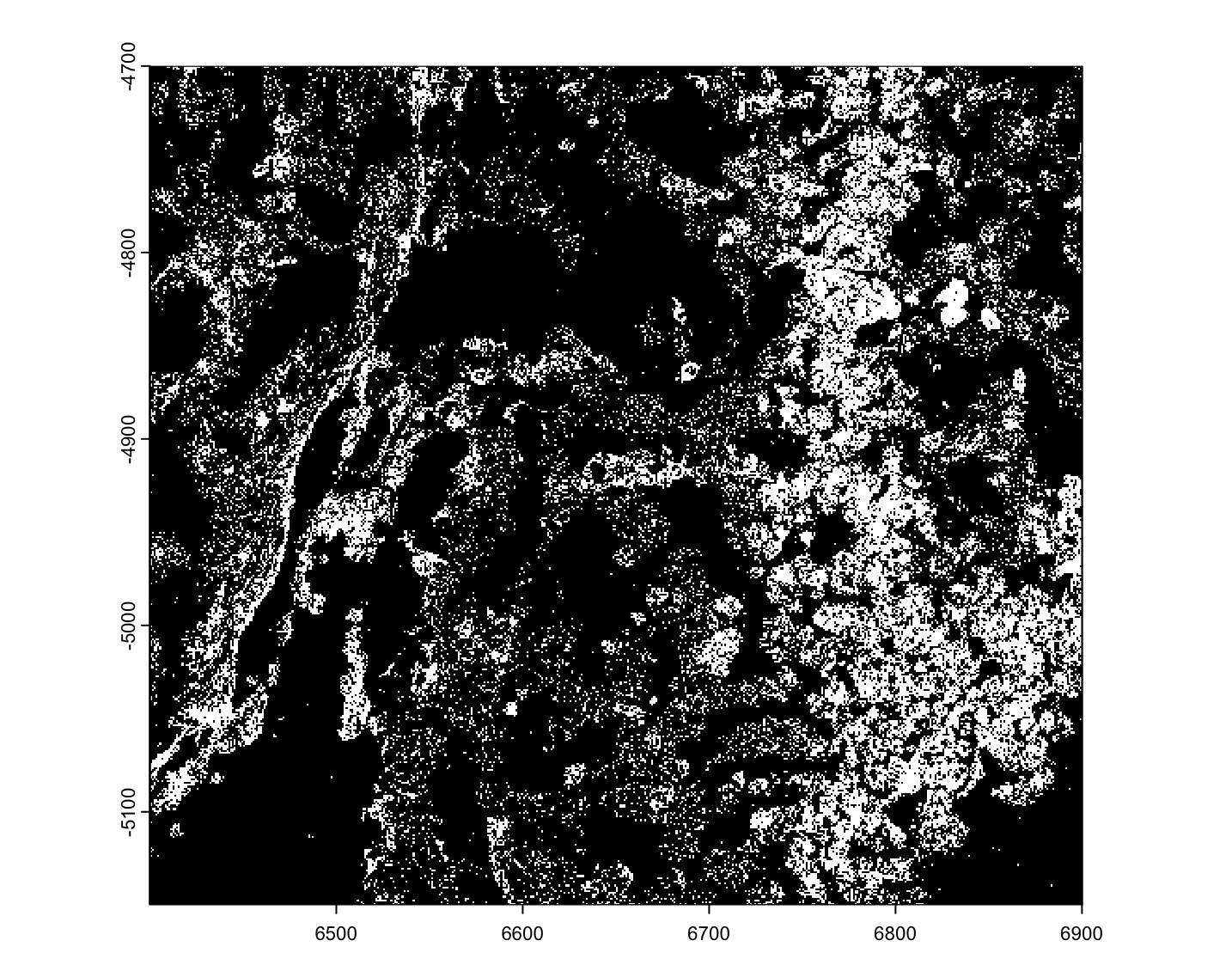
Figure 6.3: Example mini MERSCOPE transcripts data
mini_viz <- createGiottoObjectSubcellular(
  gpolygons = mini_viz_poly,
  gpoints = viz_gpoints
)

instructions(mini_viz, "return_plot") <- FALSE

force(mini_viz)
An object of class giotto
>Active spat_unit: cell
>Active feat_type: rna
[SUBCELLULAR INFO]
polygons : cell
features : rna
[AGGREGATE INFO]
Use objHistory() to see steps and params used# calculate centroids
mini_viz <- addSpatialCentroidLocations(mini_viz)
# create aggregated information
mini_viz <- calculateOverlap(mini_viz)
mini_viz <- overlapToMatrix(mini_viz)
spatFeatPlot2D(
mini_viz,
feats = c("Grm4", "Gfap"),
expression_values = "raw",
point_size = 2.5,
gradient_style = "sequential",
background_color = "black"
)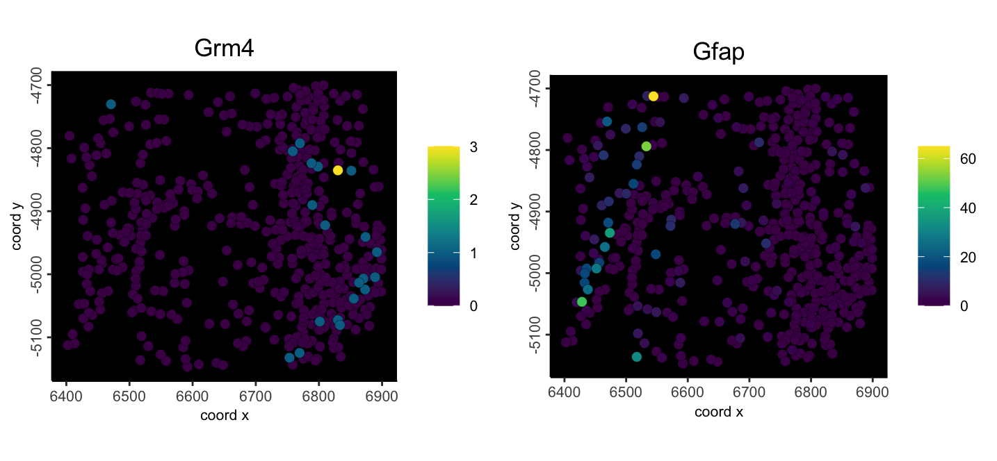
Figure 6.4: Example mini MERSCOPE aggregated feature counts
6.5 From piece-wise
You can also piece-wise assemble an object independently of one of the 2 previously shown convenience functions.
g <- giotto() # initialize empty gobject

g <- setGiotto(g, mini_viz_poly)

g <- setGiotto(g, viz_gpoints)

force(g)
An object of class giotto
>Active spat_unit: cell
>Active feat_type: rna
[SUBCELLULAR INFO]
polygons : cell
features : rna
[AGGREGATE INFO]
Use objHistory() to see steps and params usedThis is essentially the same object as the one created through createGiottoObjectSubcellular() earlier.
6.6 Using convenience functions for popular technologies (Vizgen, Xenium, CosMx, …)
There are also several convenience functions we provide for loading in data from popular platforms. These functions take care of reading the expected output folder structures, auto-detecting where needed data items are, formatting items for ingestion, then object creation. Many of these will be touched on later during other sessions.
createGiottoVisiumObject()
createGiottoVisiumHDObject()
createGiottoXeniumObject()
createGiottoCosMxObject()
createGiottoMerscopeObject()
6.7 Plotting
6.7.1 Subobject plotting
Giotto has several spatial plotting functions. At the lowest level, you directly call plot() on several subobjects in order to see what they look like, particularly the ones containing spatial info. Here we load several mini subobjects which are taken from the vizgen MERSCOPE mini dataset. To see which mini objects are available for independent loading with GiottoData::loadSubObjectMini(), you can run GiottoData::listSubobjectMini()
gpoints <- GiottoData::loadSubObjectMini("giottoPoints")

plot(gpoints)

plot(gpoints, dens = TRUE, col = getColors("magma", 255))

plot(gpoints, raster = FALSE)

plot(gpoints, feats = c("Grm4", "Gfap"))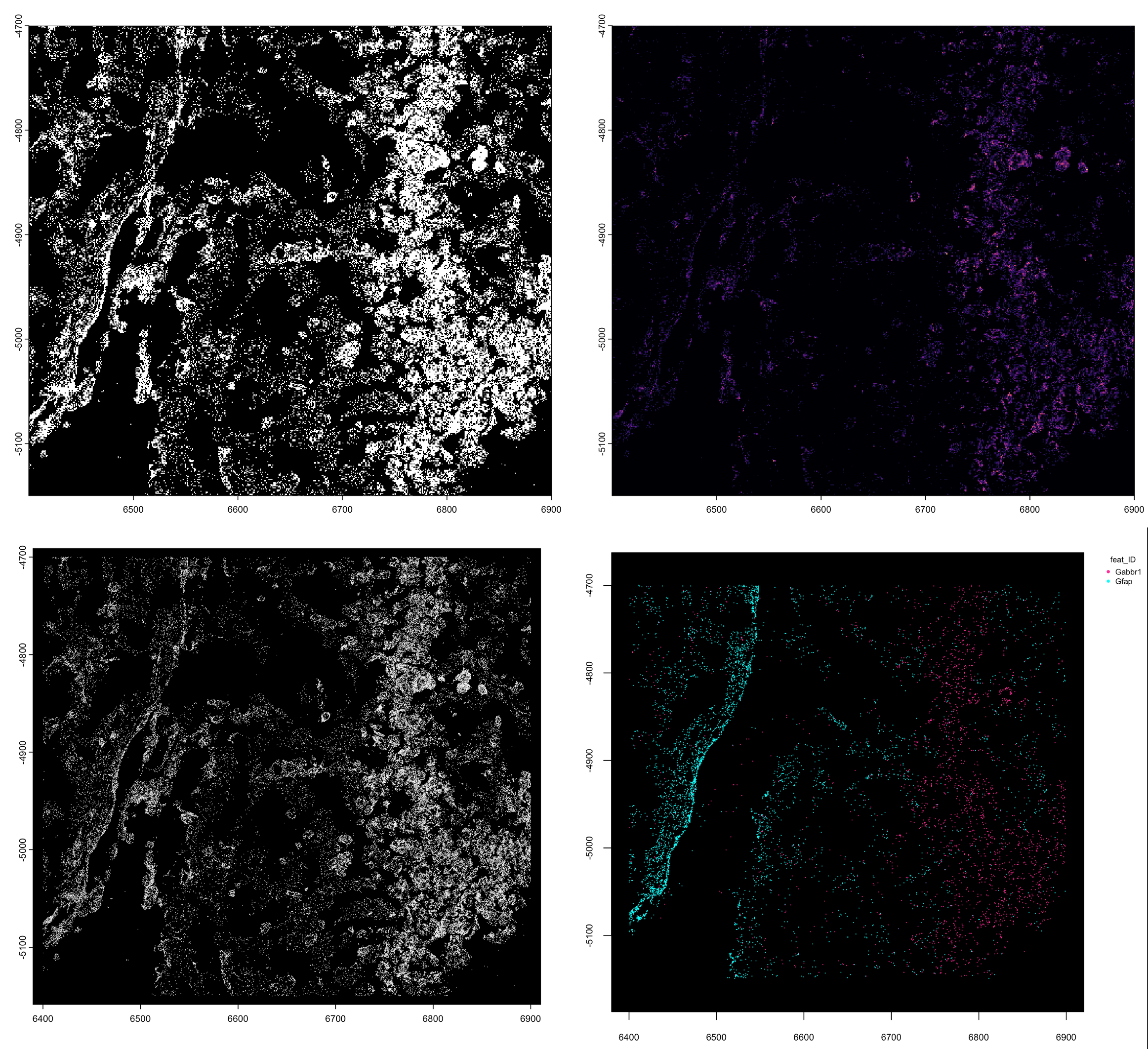
Figure 6.5: giottoPoints plots. Rasterized (top left), Rasterized and colored with ‘magma’ color scale by density (top right), Non-rasterized (bottom left), Plotting specifically 2 features (bottom right)
gpoly <- GiottoData::loadSubObjectMini("giottoPolygon")

plot(gpoly)

plot(gpoly, type = "centroid")

plot(gpoly, max_poly = 10)
Figure 6.6: giottoPolygon plots. default (left), plotting centroids (middle), auto changing to centroids after there are more polygons to plot than max_poly param (right)
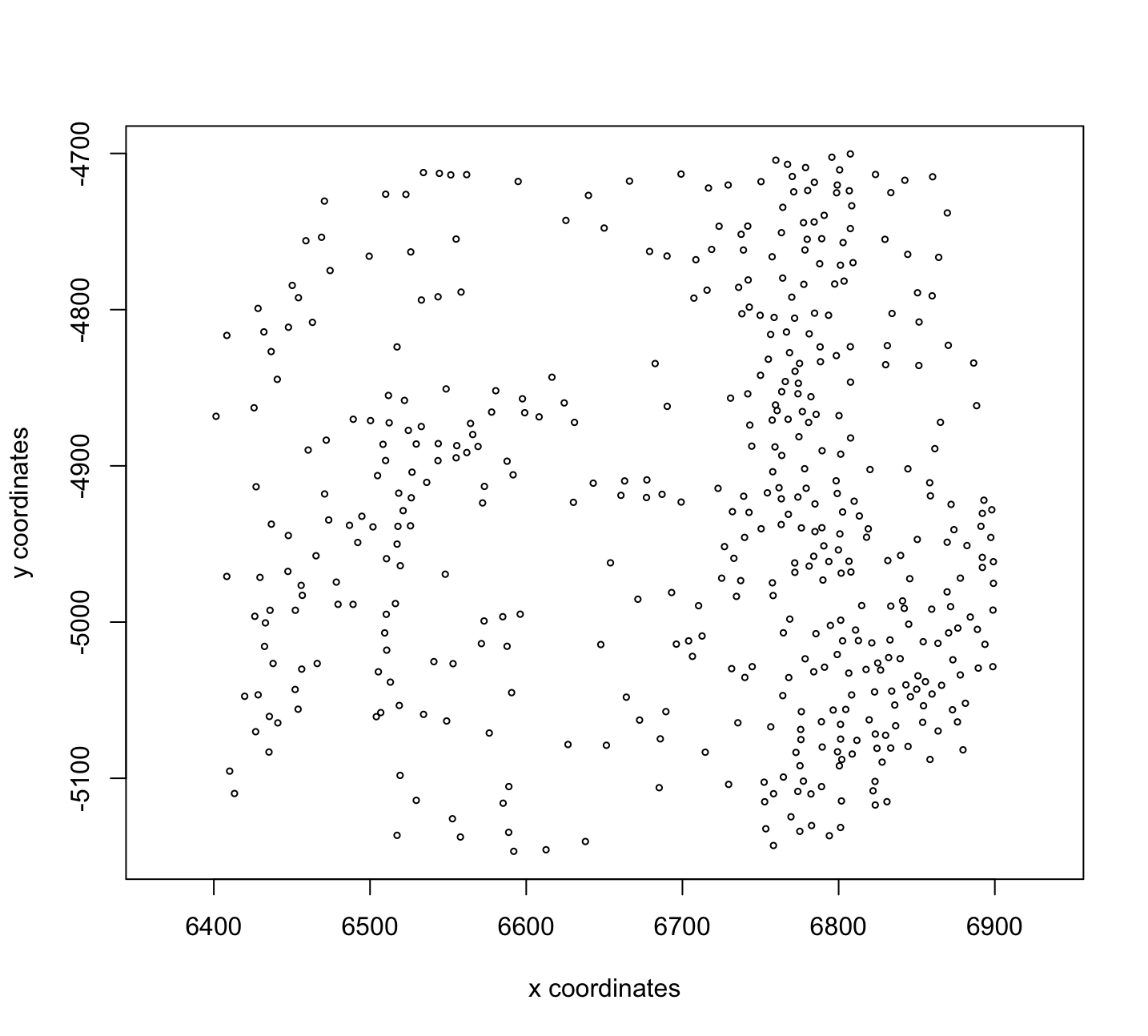
Figure 6.7: Plot of spatLocsObj
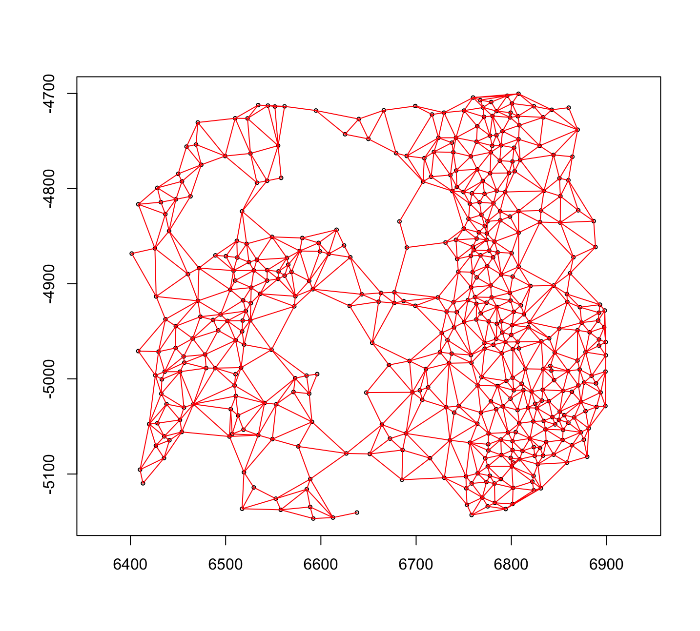
Figure 6.8: Plot of spatialNetworkObj
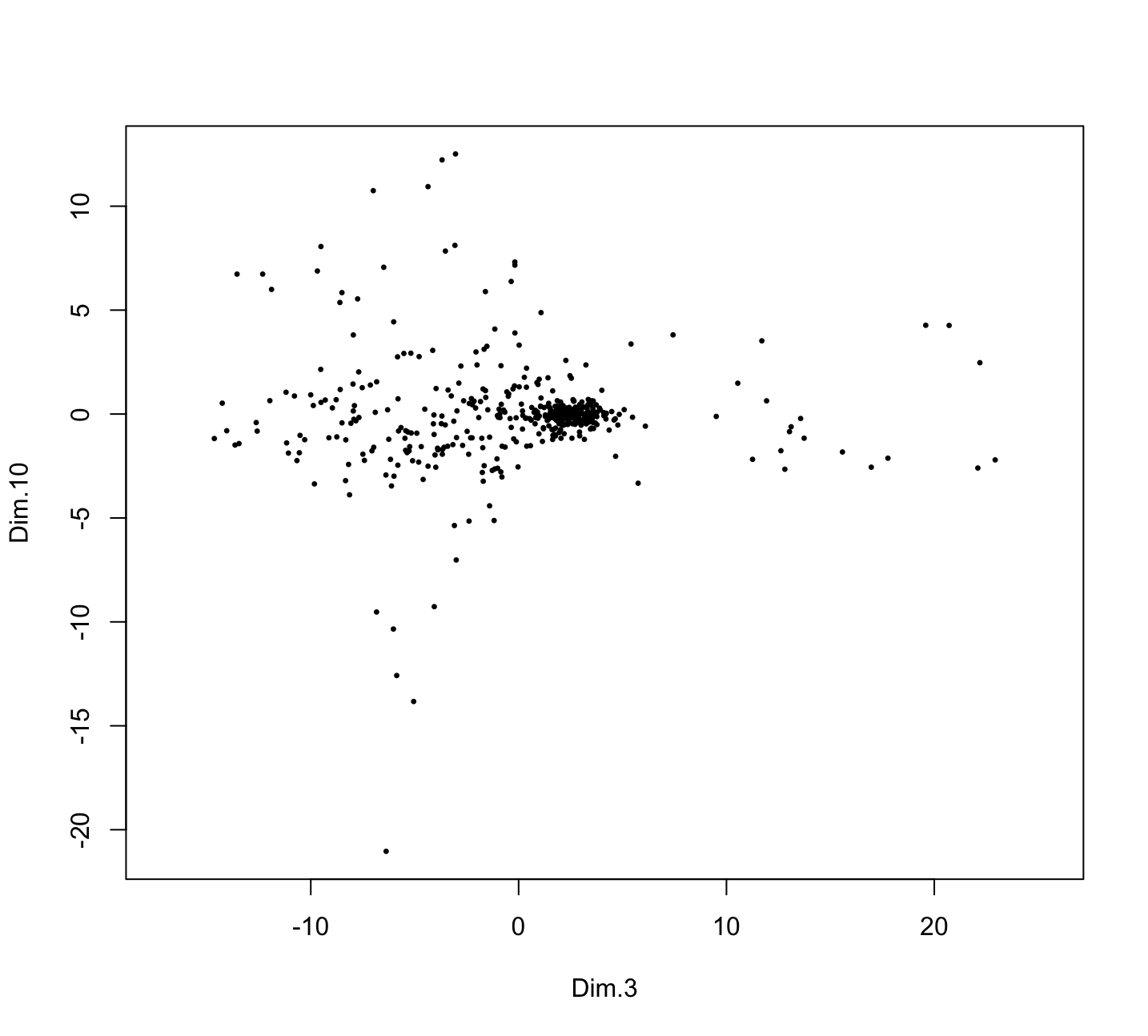
Figure 6.9: Plot of PCA dimObj showing the 3rd and 10th PCs
6.7.2 Additive subobject plotting
These base plotting functions inherit from terra::plot(). They can be used additively with more than one object.
gimg <- GiottoData::loadSubObjectMini("giottoLargeImage")

plot(gimg, col = getMonochromeColors("#5FAFFF"))

plot(gpoly, border = "maroon", lwd = 0.5, add = TRUE)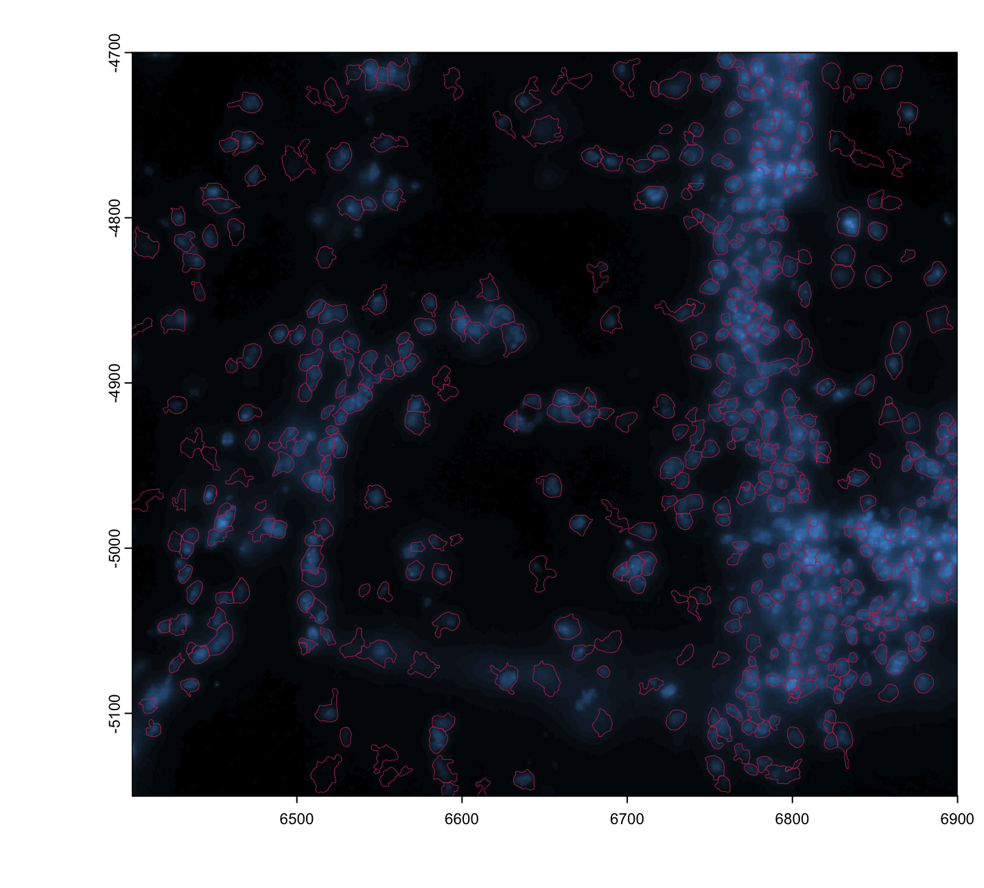
Figure 6.10: Plot image with monochrome color scaling with added polygon borders
6.7.3 Giotto object plotting
Giotto also has several ggplot2-based plotting functions that work on the whole giotto object. Here we load the vizgen mini dataset from GiottoData which contains a lot of worked through data.
6.7.3.1 Giotto spatial plot functions
spatPlot() - standard centroid-based plotting geared towards metadata plotting
g <- GiottoData::loadGiottoMini("vizgen")

activeSpatUnit(g) <- "aggregate" # set default spat_unit to the one with lots of results

force(g)
An object of class giotto
>Active spat_unit: aggregate
>Active feat_type: rna
[SUBCELLULAR INFO]
polygons : z0 z1 aggregate
features : rna
[AGGREGATE INFO]
expression -----------------------
[z0][rna] raw
[z1][rna] raw
[aggregate][rna] raw normalized scaled pearson
spatial locations ----------------
[z0] raw
[z1] raw
[aggregate] raw
spatial networks -----------------
[aggregate] Delaunay_network kNN_network
spatial enrichments --------------
[aggregate][rna] cluster_metagene
dim reduction --------------------
[aggregate][rna] pca umap tsne
nearest neighbor networks --------
[aggregate][rna] sNN.pca
attached images ------------------
images : 4 items...
Use objHistory() to see steps and params usedWhat metadata do we have in this mini object?
cell_ID nr_feats perc_feats total_expr leiden_clus
<char>    <int>      <num>      <num>       <num>
1: 240649020551054330404932383065726870513        5   1.483680   49.40986           2
2: 274176126496863898679934791272921588227       27   8.011869  191.50684           2
3: 323754550002953984063006506310071917306       23   6.824926  173.86955           4
4:  87260224659312905497866017323180367450       37  10.979228  246.04928           5
5:  17817477728742691260808256980746537959       18   5.341246  142.44520           4
---
458:   6380671372744430258754116433861320161       54  16.023739  339.24383           2
459:  75286702783716447443887872812098770697       45  13.353116  286.81011           1
460:   9677424102111816817518421117250891895       30   8.902077  211.71790           2
461:  17685062374745280598492217386845129350        5   1.483680   48.99550           2
462:  32422253415776258079819139802733069941       12   3.560831  102.52805           2
louvain_clus
<num>
1:            0
2:            3
3:            8
4:            6
5:            7
---
458:            0
459:           23
460:            3
461:           14
462:            0
We have some expression count statistics and clustering annotations already present in the object
spatPlot2D(g,
           cell_color = "leiden_clus")

spatPlot2D(g,
           cell_color = "leiden_clus",
           show_image = TRUE,
           image_name = "dapi_z0")

spatPlot2D(g,
           cell_color = "total_expr",
           color_as_factor = FALSE,
           gradient_style = "sequential")

spatPlot2D(g,
           cell_color = "leiden_clus",
           group_by = "leiden_clus")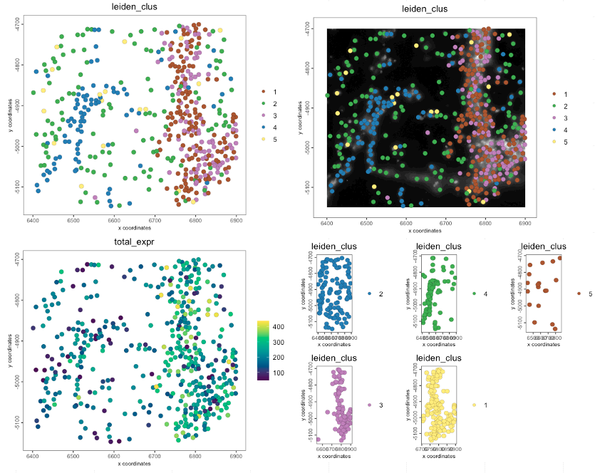
Figure 6.11: Spatial plots
spatCellPlot() - centroid-based plotting for spatial enrichment values
We have a cluster_metagene enrichment already made in the object that is a numerical measure of how much each of the cells map to the leiden clusters we have above
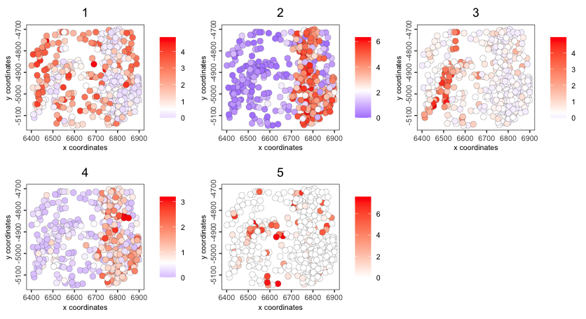
Figure 6.12: Spatial cell plot of cluster_metagene spatial enrichments
spatCellPlot2D(g,
               spat_enr_names = "cluster_metagene",
               cell_annotation_values = as.character(1:5),
               cell_color_gradient = "magma",
               background_color = "black")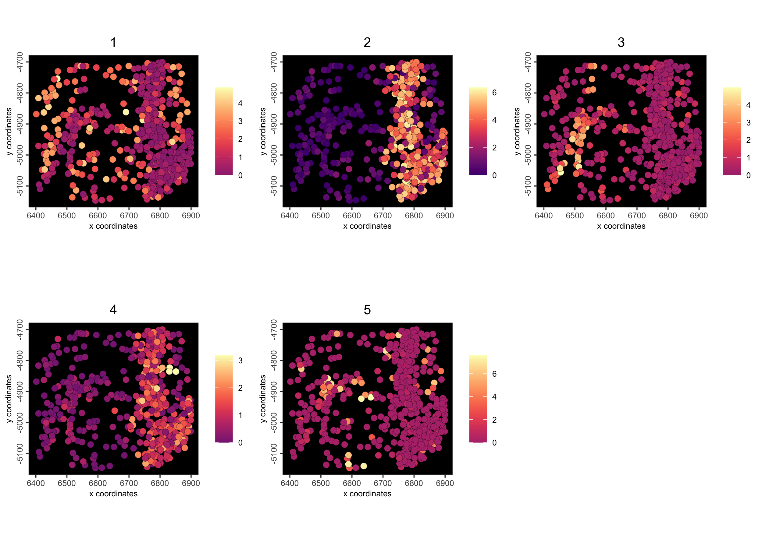
Figure 6.13: Spatial cell plot of cluster_metagene spatial enrichments
spatFeatPlot() - centroid-based plotting for feature expression plotting
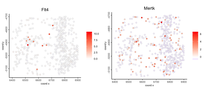
Figure 6.14: Spatial feature expression plot of normalized Flt4 (left) and Mertk expression (right)
spatInSituPlotPoints() - subcellular plotting with support for transcript points and polygons
spatInSituPlotPoints(g,
                     feats = list(rna = c("Flt4", "Mertk", "Gfap")), # this should be a named list
                     point_size = 0.5,
                     polygon_fill = "total_expr",
                     polygon_fill_as_factor = FALSE,
                     polygon_fill_gradient_style = "sequential",
                     polygon_alpha = 0.5,
                     plot_last = "points",
                     show_image = TRUE
)

# without overlaps
spatInSituPlotPoints(g,
                     feats = list(rna = c("Flt4", "Mertk", "Gfap")), # this should be a named list
                     point_size = 0.5,
                     use_overlap = FALSE,
                     polygon_fill = "total_expr",
                     polygon_fill_as_factor = FALSE,
                     polygon_fill_gradient_style = "sequential",
                     polygon_alpha = 0.5,
                     plot_last = "points",
                     show_image = TRUE
)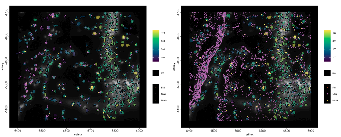
Figure 6.15: Points and polygons subcellular plot with 3 transcript species plotted, polygons colored as number of detected transcripts, and dapi image plotted. Left is with only the points overlapped by polygons, right is with all points
6.7.3.2 Giotto expression space plot functions
dimPlot() - dimension reduction plotting
Also has more specific functions for PCA plotPCA(), UMAP plotUMAP(), tSNE plotTSNE() results.
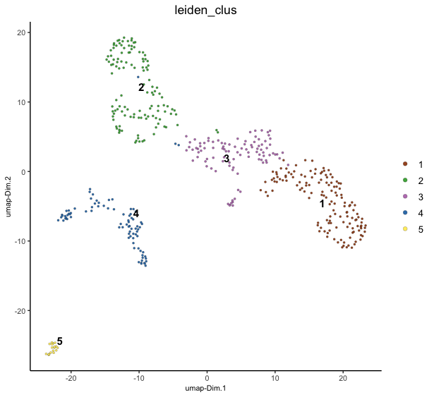
Figure 6.16: UMAP projection with leiden clustering colors
6.7.3.3 Giotto common plotting args
gradient_style- Should the gradient be of ‘divergent’ or ‘sequential’ styles?color_as_factor- Is annotation value a numerical or factor/categorical based item to plot.cell_color_code- What color mapping to providecell_color- What column of information to use when plotting (metadata, expression, etc.)point_shape- Either ‘border’ or ‘no_border’ to draw on the points.
6.8 Subsetting
6.8.1 ID subsetting
Subset the giotto object for a random 300 cell IDs
[1] 462[1] 337 462instructions(g, "cell_color_c_pal") <- "viridis"
instructions(g, "poly_color_c_pal") <- "viridis"
set.seed(1234)
gsubset <- subsetGiotto(g,
cell_ids = sample(spatIDs(g), 300))[1] 300spatPlot(g,
cell_color = "total_expr",
color_as_factor = FALSE,
background_color = "black")
spatPlot(gsubset,
cell_color = "total_expr",
color_as_factor = FALSE,
background_color = "black")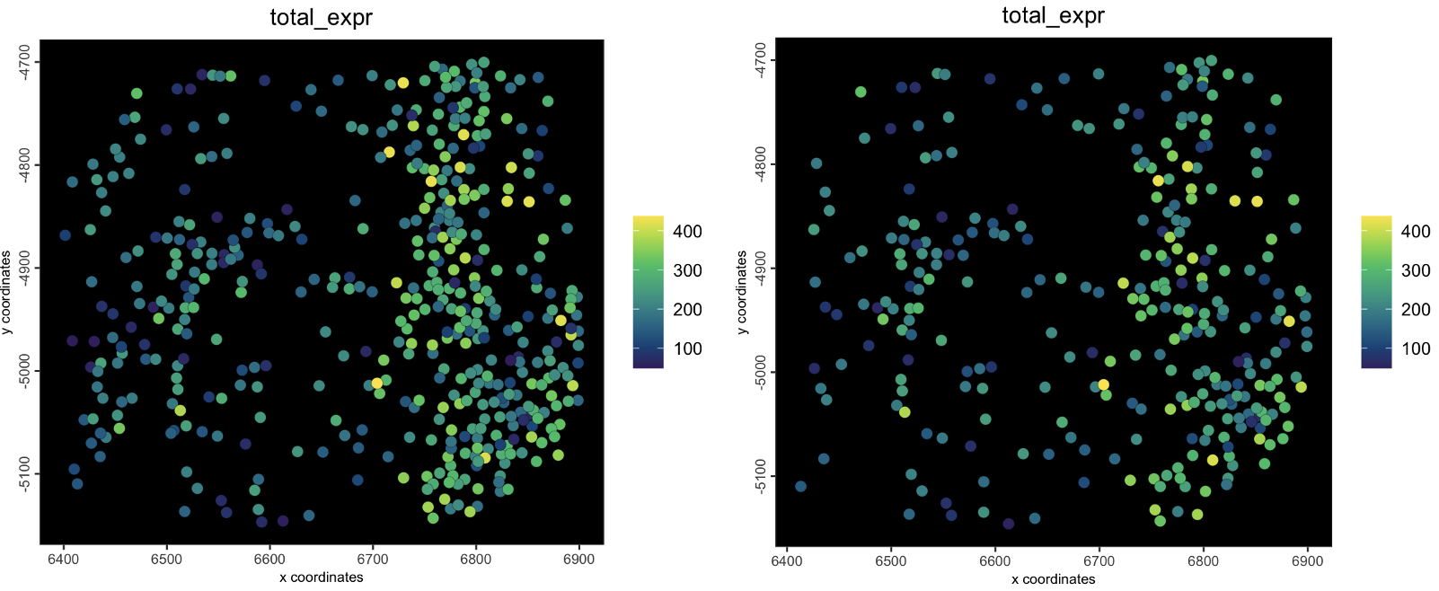
Figure 6.17: plot showing starting object (left) and subset object (right)
6.8.2 Coordinate-based subsetting
spatPlot(gsubsetlocs,
         cell_color = "total_expr",
         color_as_factor = FALSE,
         background_color = "black")

spatInSituPlotPoints(gsubsetlocs,
                     polygon_fill = "total_expr",
                     polygon_fill_as_factor = FALSE)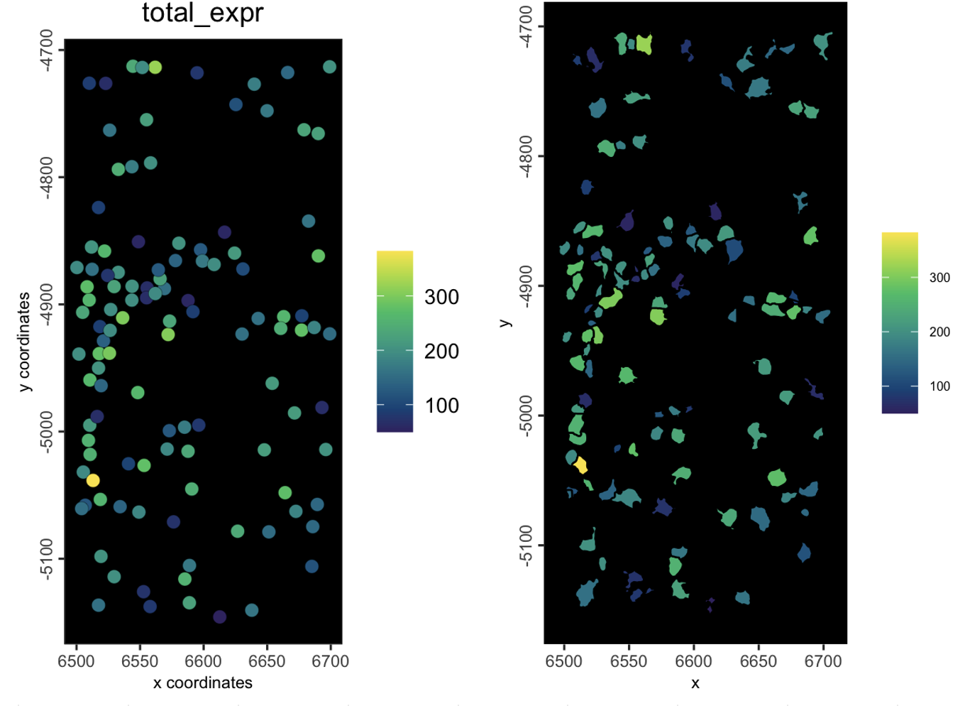
Figure 6.18: plot showing starting object (left) and subset object (right)