8 Visium Part II
Joselyn Cristina Chávez Fuentes
August 6th 2024
8.2 Differential expression
8.2.1 Gini markers
The Gini method identifies genes that are very selectively expressed in a specific cluster, however not always expressed in all cells of that cluster. In other words, highly specific but not necessarily sensitive at the single-cell level.
- Calculate the top marker genes per cluster using the gini method.
gini_markers <- findMarkers_one_vs_all(gobject = visium_brain,
                                       method = "gini",
                                       expression_values = "normalized",
                                       cluster_column = "leiden_clus",
                                       min_feats = 10)

topgenes_gini <- gini_markers[, head(.SD, 2), by = "cluster"]$feats- Visualize
Plot the normalized expression distribution of the top expressed genes.
violinPlot(visium_brain,
           feats = unique(topgenes_gini),
           cluster_column = "leiden_clus",
           strip_text = 6,
           strip_position = "right",
           save_param = list(base_width = 5, base_height = 30))
Figure 8.1: Violin plot showing the top gini genes normalized expression.
Use the cluster IDs to create a heatmap with the normalized expression of the top expressed genes per cluster.
plotMetaDataHeatmap(visium_brain,
                    selected_feats = unique(topgenes_gini),
                    metadata_cols = "leiden_clus",
                    x_text_size = 10, y_text_size = 10)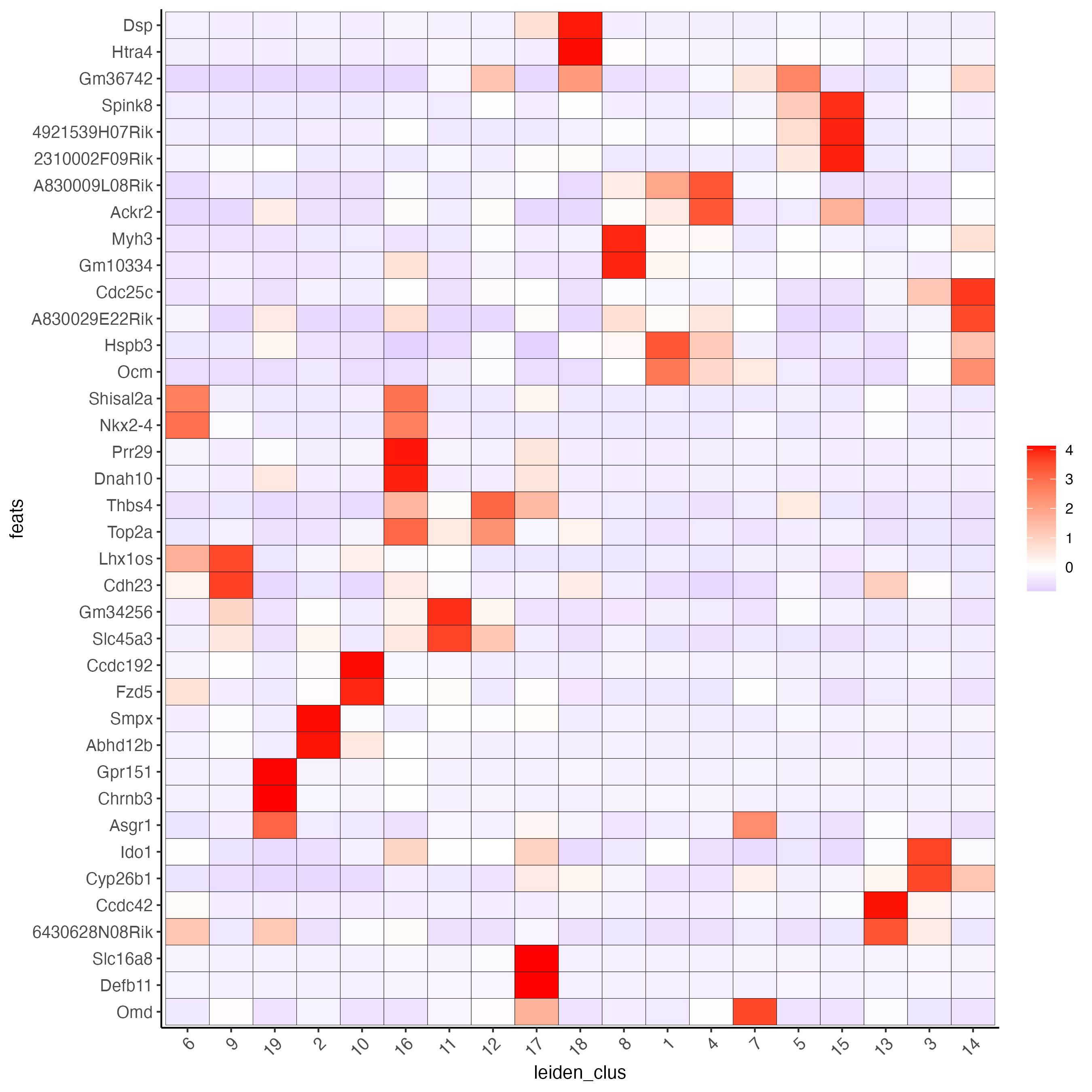
Figure 8.2: Heatmap showing the top gini genes normalized expression per Leiden cluster.
Visualize the scaled expression spatial distribution of the top expressed genes across the sample.
dimFeatPlot2D(visium_brain,
              expression_values = "scaled",
              feats = sort(unique(topgenes_gini)),
              cow_n_col = 5,
              point_size = 1,
              save_param = list(base_width = 15, base_height = 20))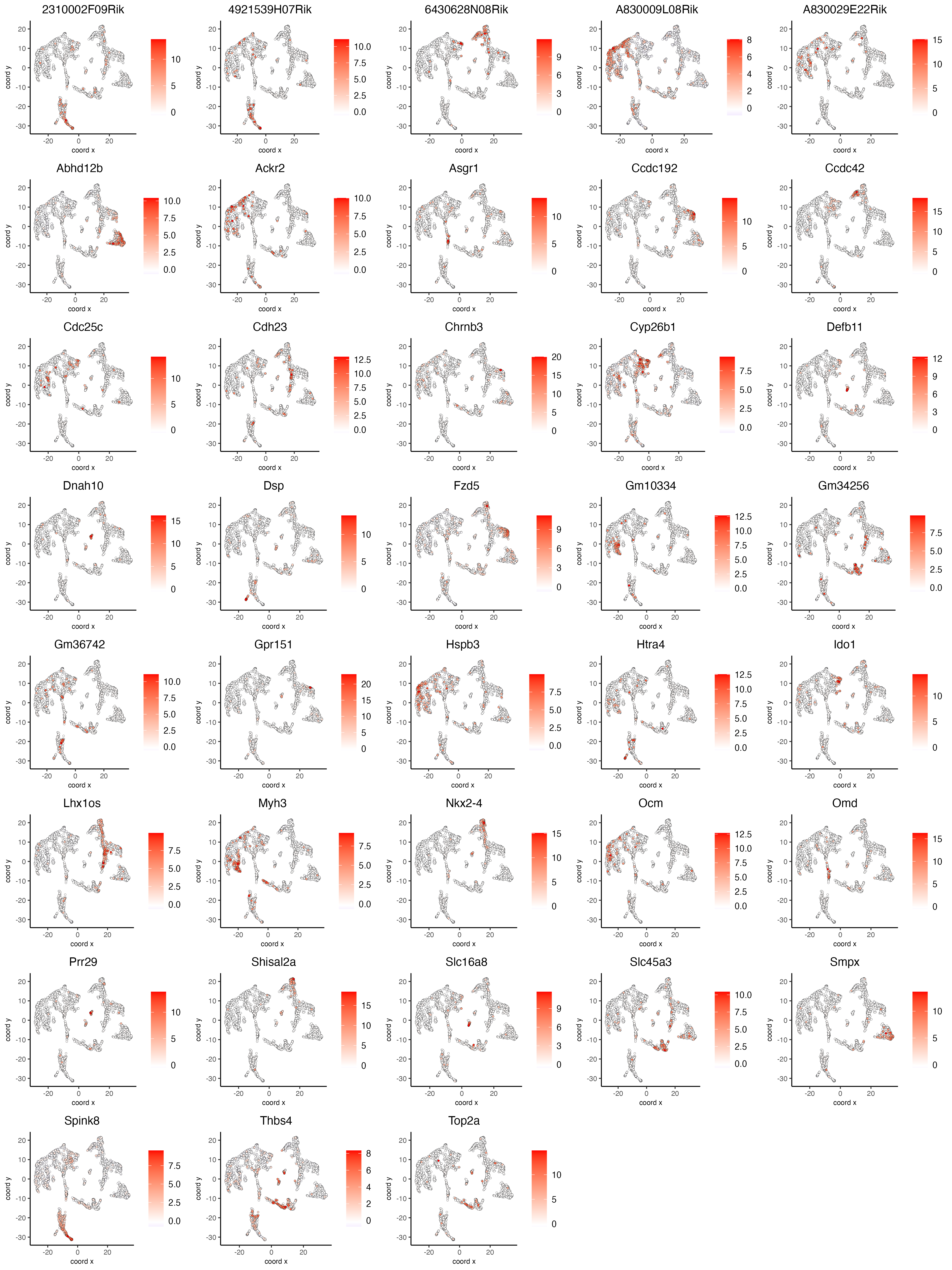
Figure 8.3: Spatial distribution of the top gini genes scaled expression.
8.2.2 Scran markers
The Scran method is preferred for robust differential expression analysis, especially when addressing technical variability or differences in sequencing depth across spatial locations. [redo]
- Calculate the top marker genes per cluster using the scran method
scran_markers <- findMarkers_one_vs_all(gobject = visium_brain,
                                       method = "scran",
                                       expression_values = "normalized",
                                       cluster_column = "leiden_clus",
                                       min_feats = 10)

topgenes_scran <- scran_markers[, head(.SD, 2), by = "cluster"]$feats- Visualize
Plot the normalized expression distribution of the top expressed genes.
violinPlot(visium_brain,
           feats = unique(topgenes_scran),
           cluster_column = "leiden_clus",
           strip_text = 6,
           strip_position = "right",
           save_param = list(base_width = 5, base_height = 30))
Figure 8.4: Violin plot of the top scran genes normalized expression.
Use the cluster IDs to create a heatmap with the normalized expression of the top expressed genes per cluster.
plotMetaDataHeatmap(visium_brain,
                    selected_feats = unique(topgenes_scran),
                    metadata_cols = "leiden_clus",
                    x_text_size = 10, y_text_size = 10)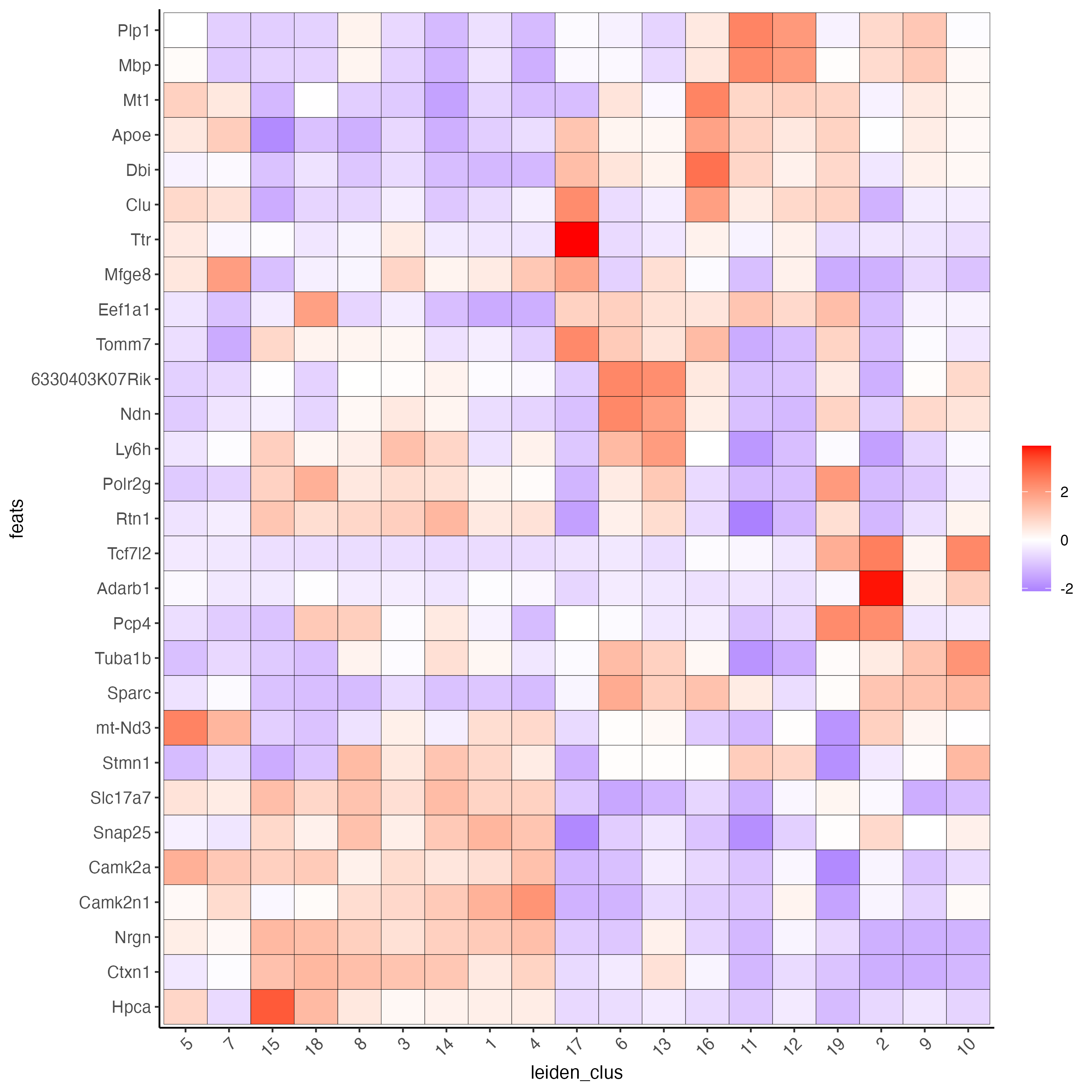
Figure 8.5: Heatmap showing the top scran genes normalized expression per Leiden cluster.
Visualize the scaled expression spatial distribution of the top expressed genes across the sample.
dimFeatPlot2D(visium_brain,
              expression_values = "scaled",
              feats = sort(unique(topgenes_scran)),
              cow_n_col = 5,
              point_size = 1,
              save_param = list(base_width = 20, base_height = 20))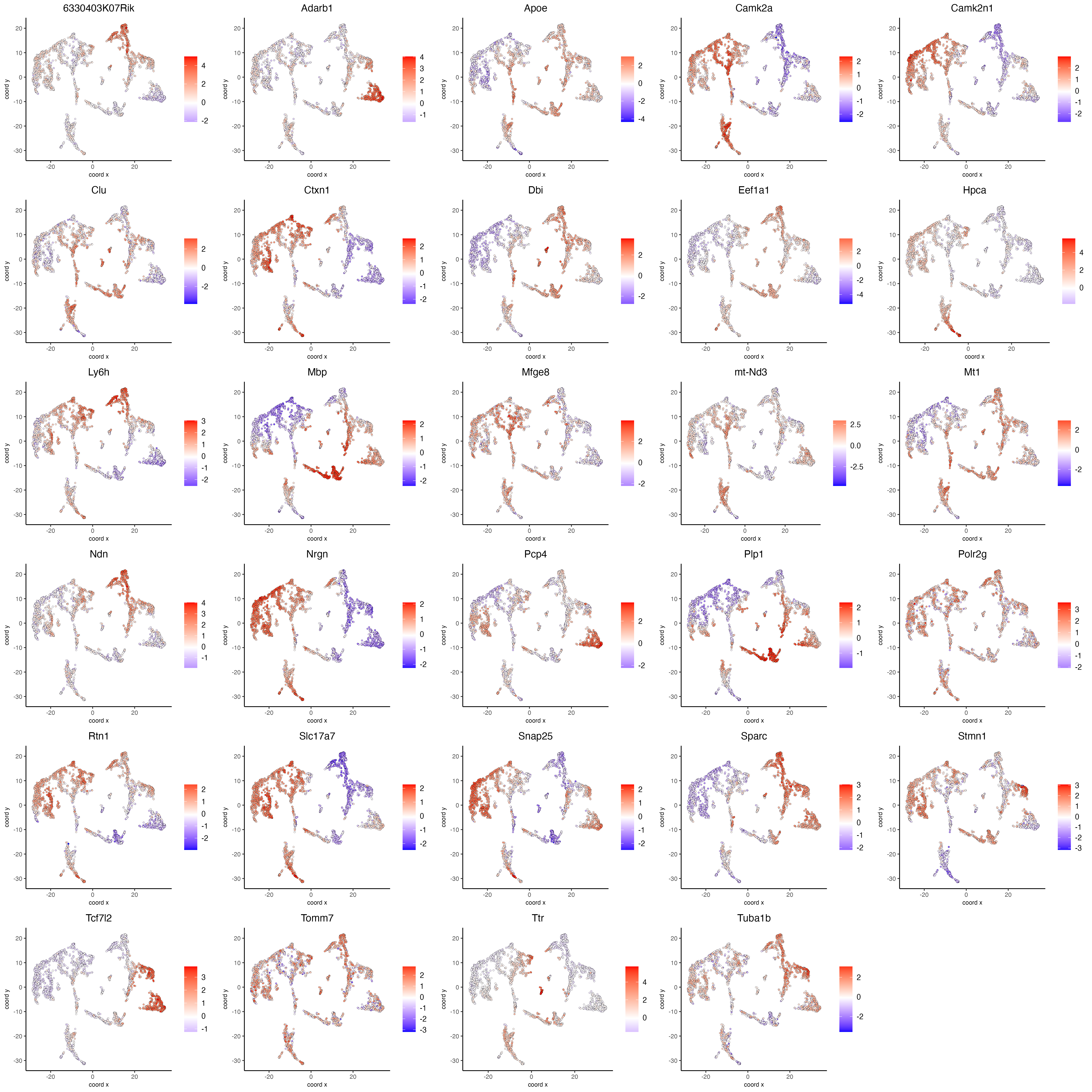
Figure 8.6: Spatial distribution of the top scran genes scaled expression.
In practice, it is often beneficial to apply both Gini and Scran methods and compare results for a more complete understanding of differential gene expression across clusters.
8.3 Enrichment & Deconvolution
Visium spatial transcriptomics does not provide single-cell resolution, making cell type annotation a harder problem. Giotto provides several ways to calculate enrichment of specific cell-type signature gene lists.
- Download the single-cell dataset
- Create the single-cell object and run the normalization step
results_folder <- "results/02_session1"

python_path <- NULL

instructions <- createGiottoInstructions(
    save_dir = results_folder,
    save_plot = TRUE,
    show_plot = FALSE,
    python_path = python_path
)

sc_expression <- "data/02_session1/brain_sc_expression_matrix.txt.gz"
sc_metadata <- "data/02_session1/brain_sc_metadata.csv"

giotto_SC <- createGiottoObject(expression = sc_expression,
                                instructions = instructions)

giotto_SC <- addCellMetadata(giotto_SC,
                             new_metadata = data.table::fread(sc_metadata))

giotto_SC <- normalizeGiotto(giotto_SC)
8.3.1 PAGE/Rank
Parametric Analysis of Gene Set Enrichment (PAGE) and Rank enrichment both aim to determine whether a predefined set of genes show statistically significant differences in expression compared to other genes in the dataset.
- Calculate the cell type markers
markers_scran <- findMarkers_one_vs_all(gobject = giotto_SC,
                                        method = "scran",
                                        expression_values = "normalized",
                                        cluster_column = "Class",
                                        min_feats = 3)

top_markers <- markers_scran[, head(.SD, 10), by = "cluster"]
celltypes <- levels(factor(markers_scran$cluster)) - Create the signature matrix
sign_list <- list()

for (i in 1:length(celltypes)){
  sign_list[[i]] = top_markers[which(top_markers$cluster == celltypes[i]),]$feats
}

sign_matrix <- makeSignMatrixPAGE(sign_names = celltypes,
sign_list = sign_list)- Run the enrichment test with PAGE
- Visualize
Create a heatmap showing the enrichment of cell types (from the single-cell data annotation) in the spatial dataset clusters.
cell_types_PAGE <- colnames(sign_matrix)

plotMetaDataCellsHeatmap(gobject = visium_brain,
                         metadata_cols = "leiden_clus",
                         value_cols = cell_types_PAGE,
                         spat_enr_names = "PAGE",
                         x_text_size = 8,
                         y_text_size = 8)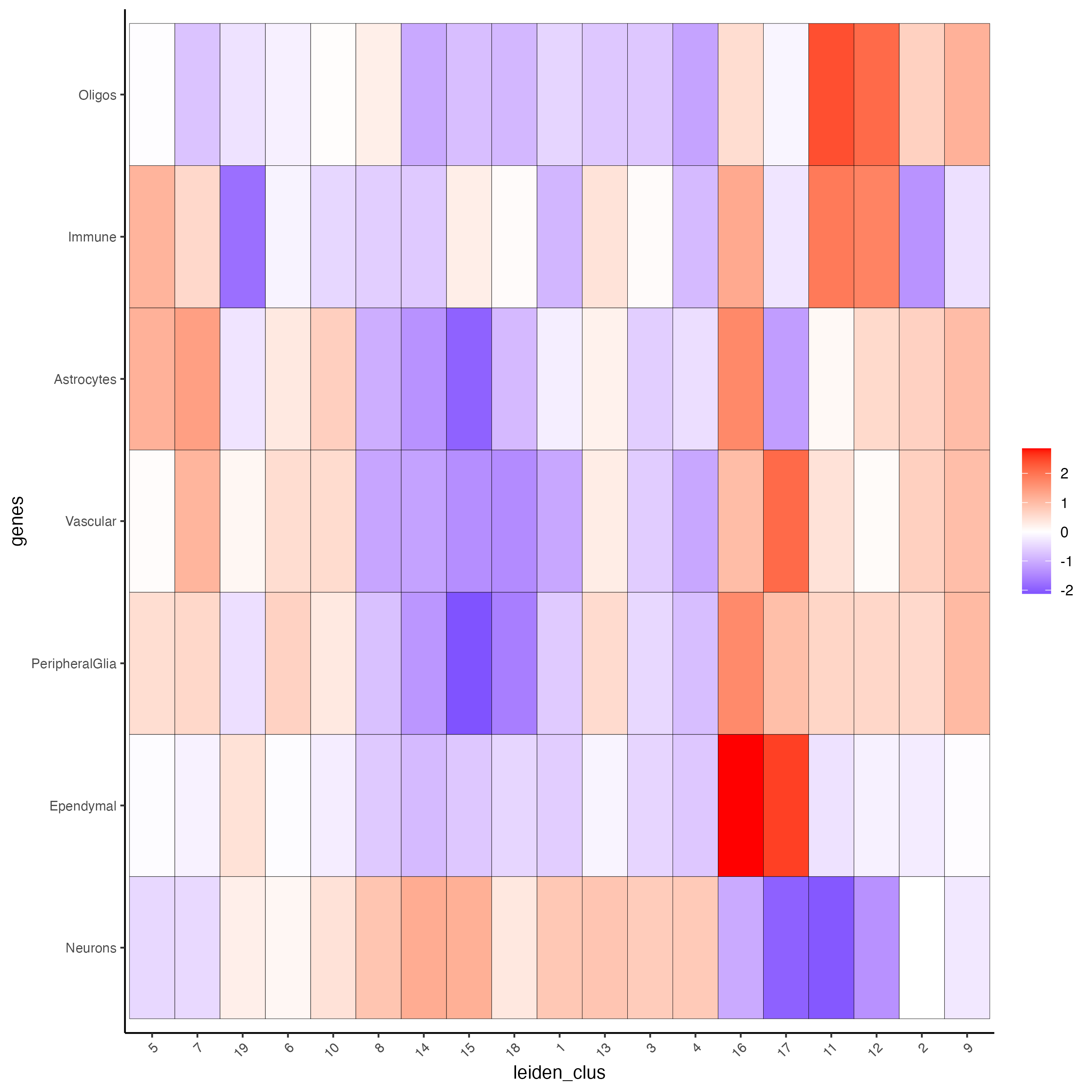
Figure 8.7: Cell types enrichment per Leiden cluster, identified using the PAGE method.
Plot the spatial distribution of the cell types.
spatCellPlot2D(gobject = visium_brain,
               spat_enr_names = "PAGE",
               cell_annotation_values = cell_types_PAGE,
               cow_n_col = 3,
               coord_fix_ratio = 1,
               point_size = 1,
               show_legend = TRUE)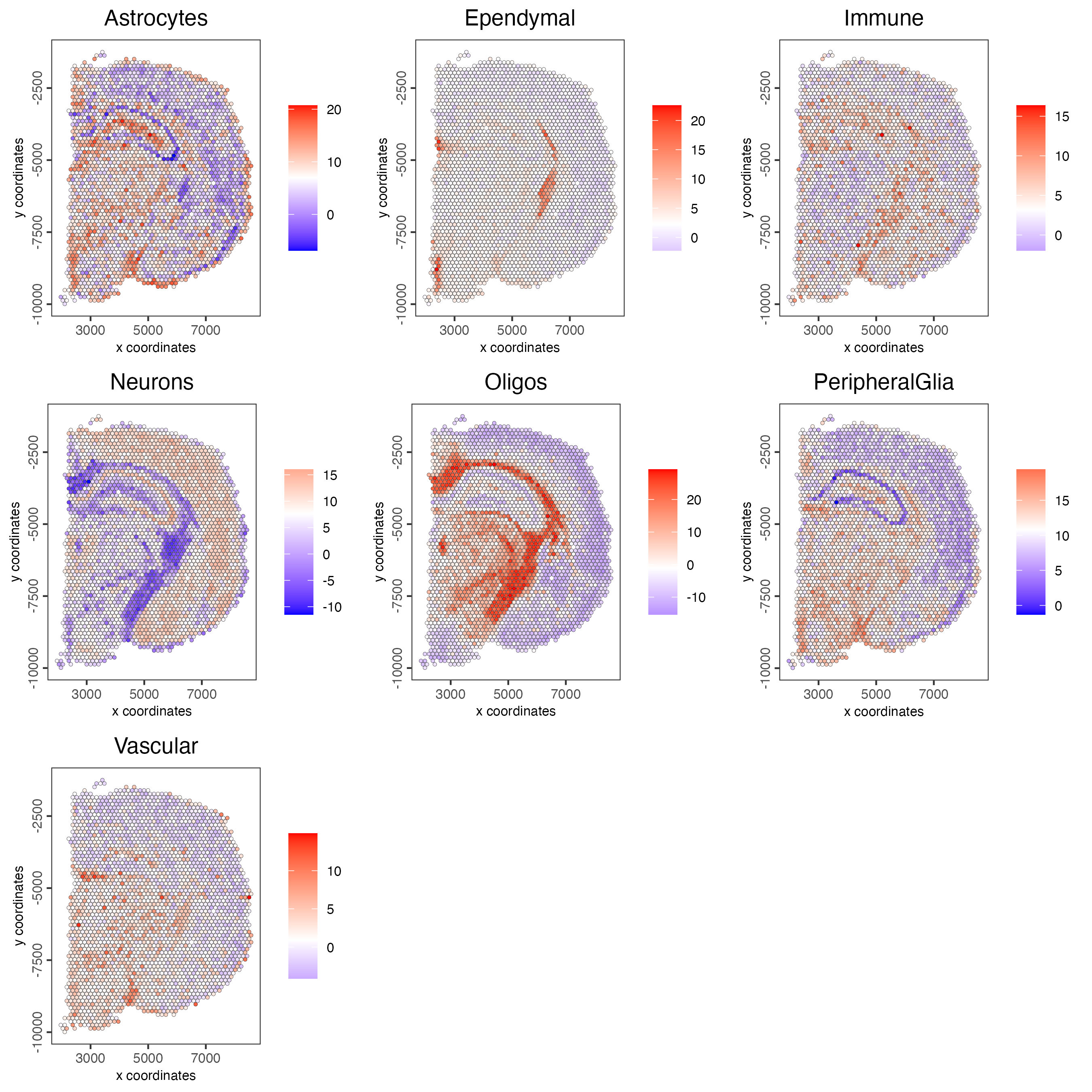
Figure 8.8: Spatial distribution of cell types identified using the PAGE method.
8.3.2 SpatialDWLS
Spatial Dampened Weighted Least Squares (DWLS) estimates the proportions of different cell types across spots in a tissue.
- Create the signature matrix
sign_matrix <- makeSignMatrixDWLSfromMatrix(
    matrix = getExpression(giotto_SC,
                           values = "normalized",
                           output = "matrix"),
    cell_type = pDataDT(giotto_SC)$Class,
sign_gene = top_markers$feats)- Run the DWLS Deconvolution
This step may take a couple of minutes to run.
- Visualize
Plot the DWLS deconvolution result creating with pie plots showing the proportion of each cell type per spot.
spatDeconvPlot(visium_brain,
               show_image = FALSE,
               radius = 50,
               save_param = list(save_name = "8_spat_DWLS_pie_plot"))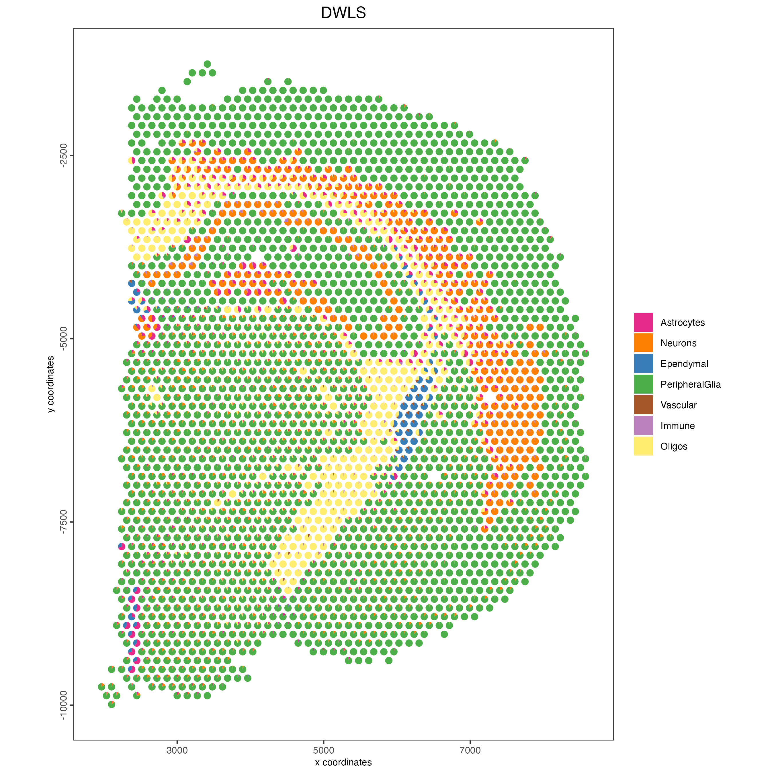
Figure 8.9: Spatial deconvolution plot showing the proportion of cell types per spot, identified using the DWLS method.
8.4 Spatial expression patterns
8.4.1 Spatial variable genes
- Create a spatial network
visium_brain <- createSpatialNetwork(gobject = visium_brain,
                                     method = "kNN",
                                     k = 6,
                                     maximum_distance_knn = 400,
                                     name = "spatial_network")

spatPlot2D(gobject = visium_brain,
           show_network= TRUE,
           network_color = "blue",
           spatial_network_name = "spatial_network")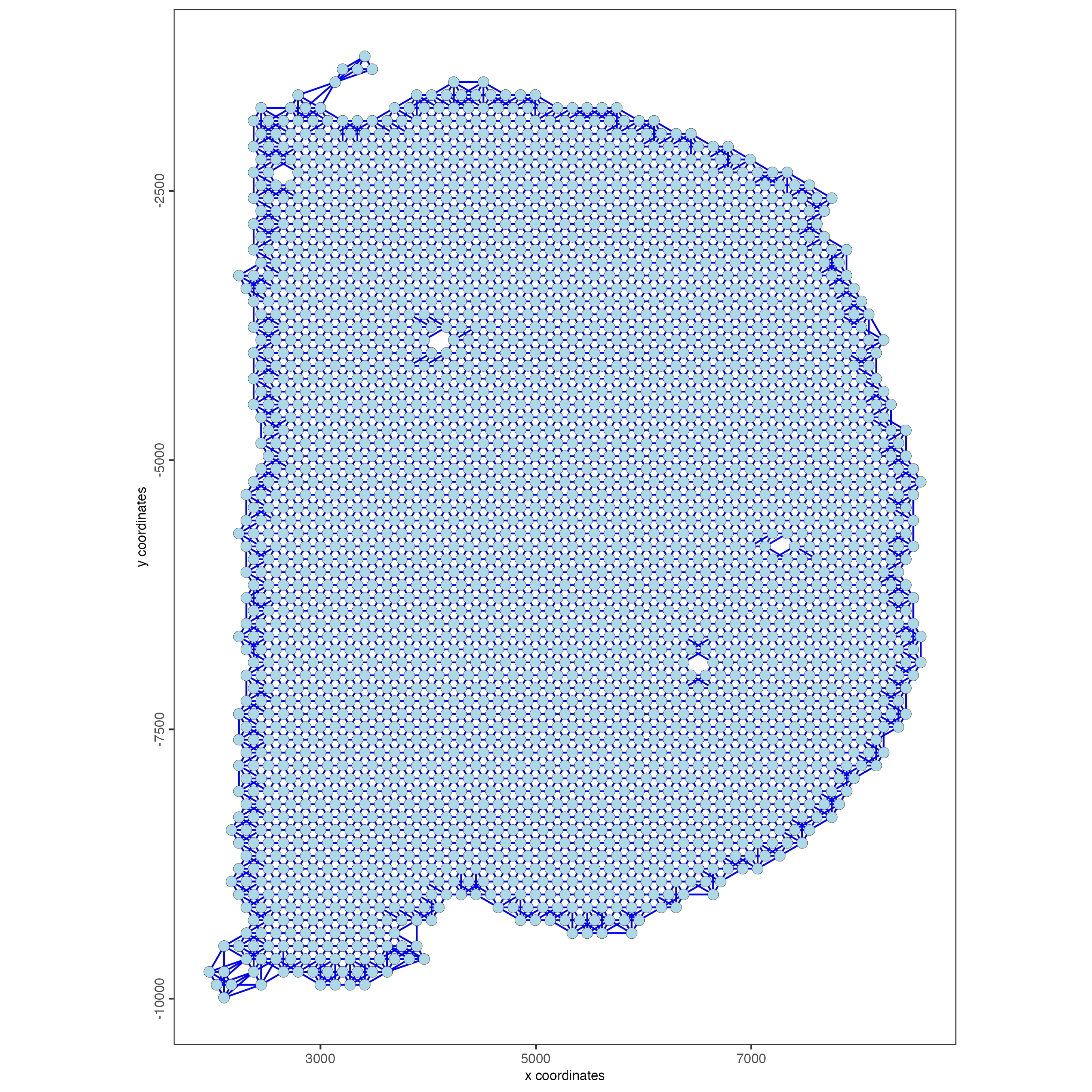
Figure 8.10: Spatial network across spots in the Visium mouse sample.
- Rank binarization
Rank the genes on the spatial dataset depending on whether they exhibit a spatial pattern location or not.
This step may take a few minutes to run.
ranktest <- binSpect(visium_brain,
                     bin_method = "rank",
                     calc_hub = TRUE,
                     hub_min_int = 5,
spatial_network_name = "spatial_network")- Visualize top results
Plot the scaled expression of genes with the highest probability of being spatial genes.
spatFeatPlot2D(visium_brain,
               expression_values = "scaled",
               feats = ranktest$feats[1:6],
               cow_n_col = 2,
               point_size = 1)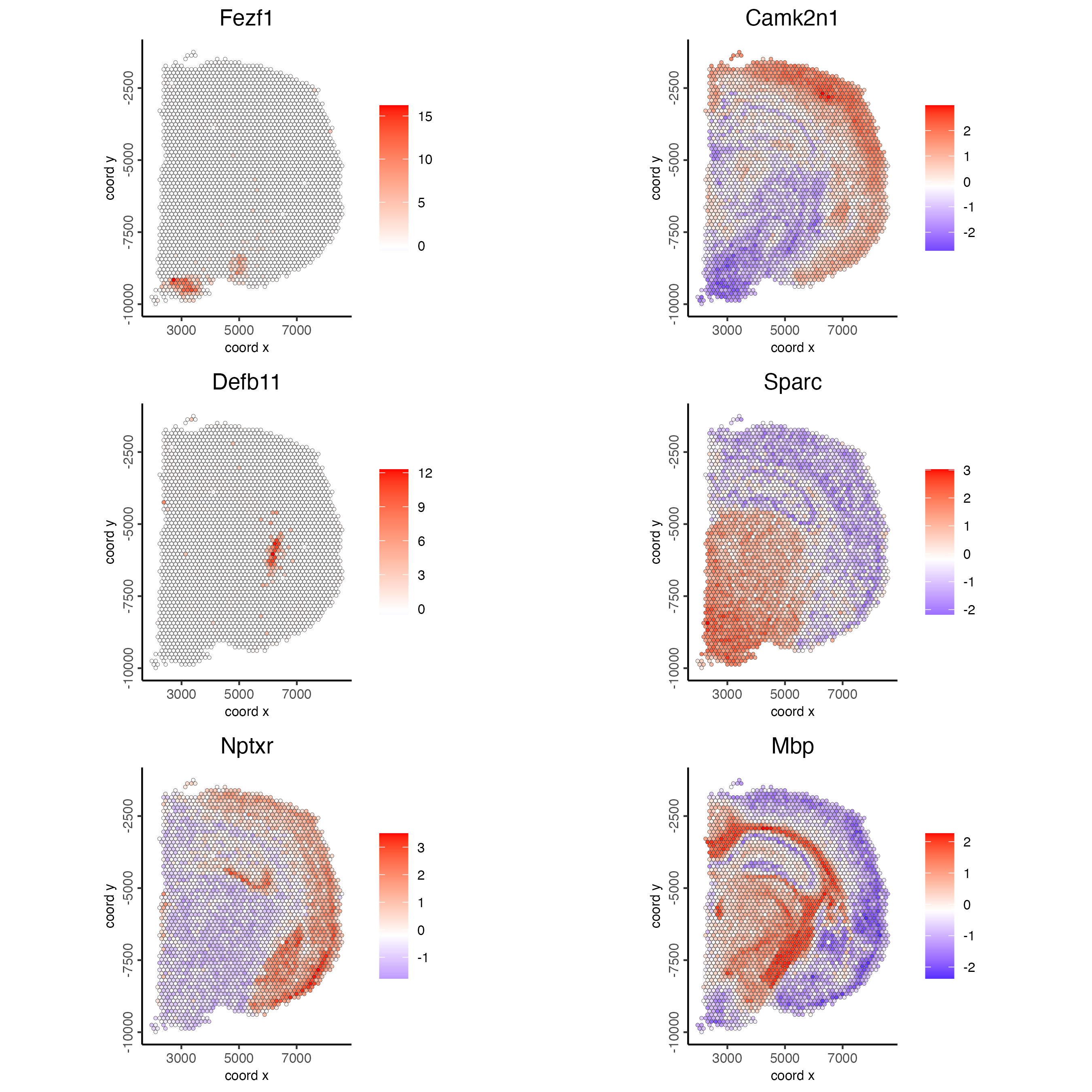
Figure 8.11: Spatial distribution of the top spatial genes scaled expression.
8.4.2 Spatial co-expression modules
- Cluster the top 500 spatial genes into 20 clusters
- Use detectSpatialCorGenes function to calculate pairwise distances between genes.
spat_cor_netw_DT <- detectSpatialCorFeats(
    visium_brain,
    method = "network",
    spatial_network_name = "spatial_network",
subset_feats = ext_spatial_genes)- Identify most similar spatially correlated genes for one gene
- Visualize
Plot the scaled expression of the 3 genes with most similar spatial patterns to Mbp.
spatFeatPlot2D(visium_brain,
               expression_values = "scaled",
               feats = top10_genes$variable[1:4],
               point_size = 1.5)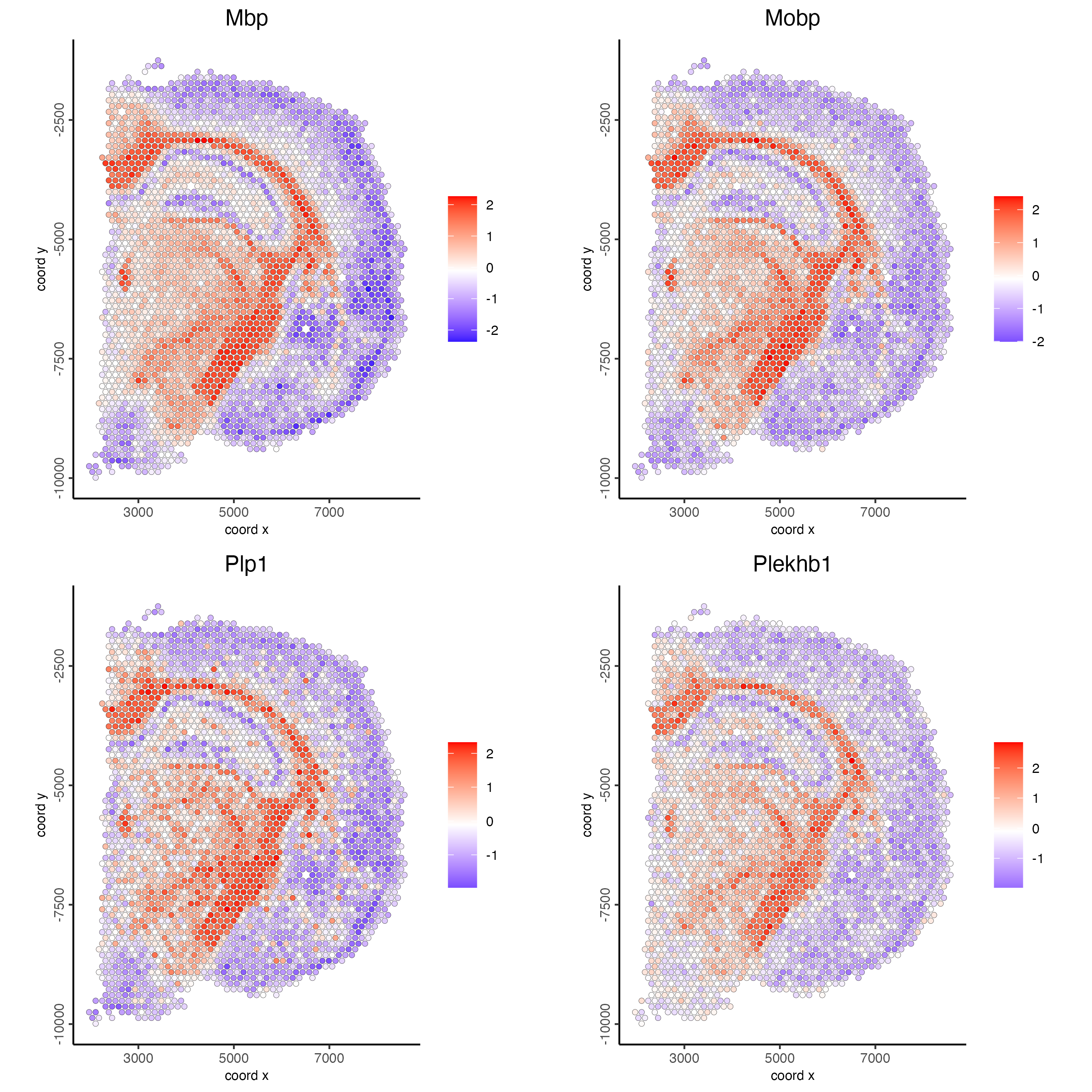
Figure 8.12: Spatial distribution of the scaled expression of 3 genes with similar spatial pattern to Mbp.
- Cluster spatial genes
- Visualize clusters
Plot the correlation of the top 500 spatial genes with their assigned cluster.
heatmSpatialCorFeats(visium_brain,
                     spatCorObject = spat_cor_netw_DT,
                     use_clus_name = "spat_netw_clus",
                     heatmap_legend_param = list(title = NULL))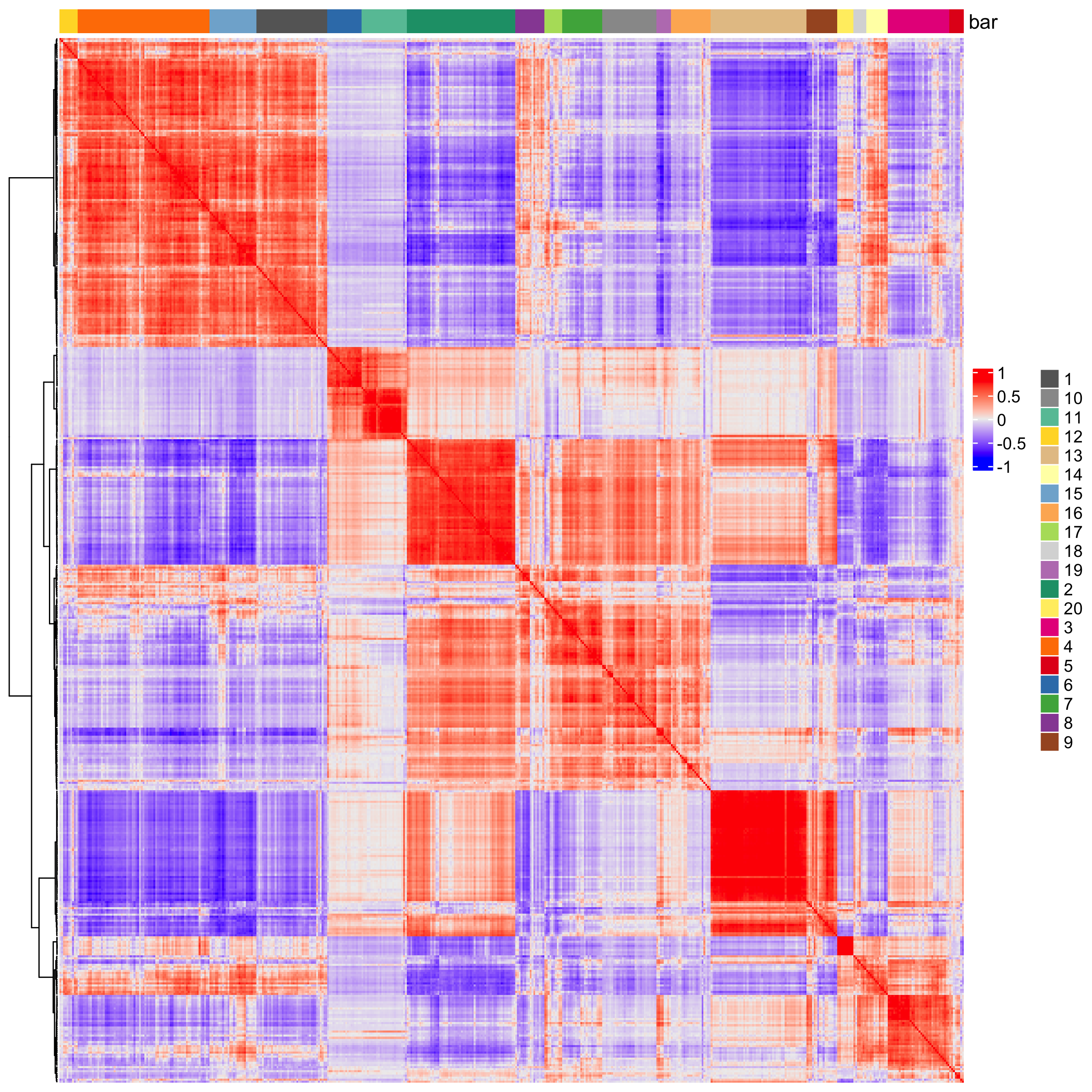
Figure 8.13: Correlations heatmap between spatial genes and correlated clusters.
- Rank spatial correlated clusters and show genes for selected clusters
netw_ranks <- rankSpatialCorGroups(
  visium_brain,
  spatCorObject = spat_cor_netw_DT,
  use_clus_name = "spat_netw_clus")
Plot the correlation and number of spatial genes in each cluster.
top_netw_spat_cluster <- showSpatialCorFeats(spat_cor_netw_DT,
                                            use_clus_name = "spat_netw_clus",
                                            selected_clusters = 6,
                                            show_top_feats = 1)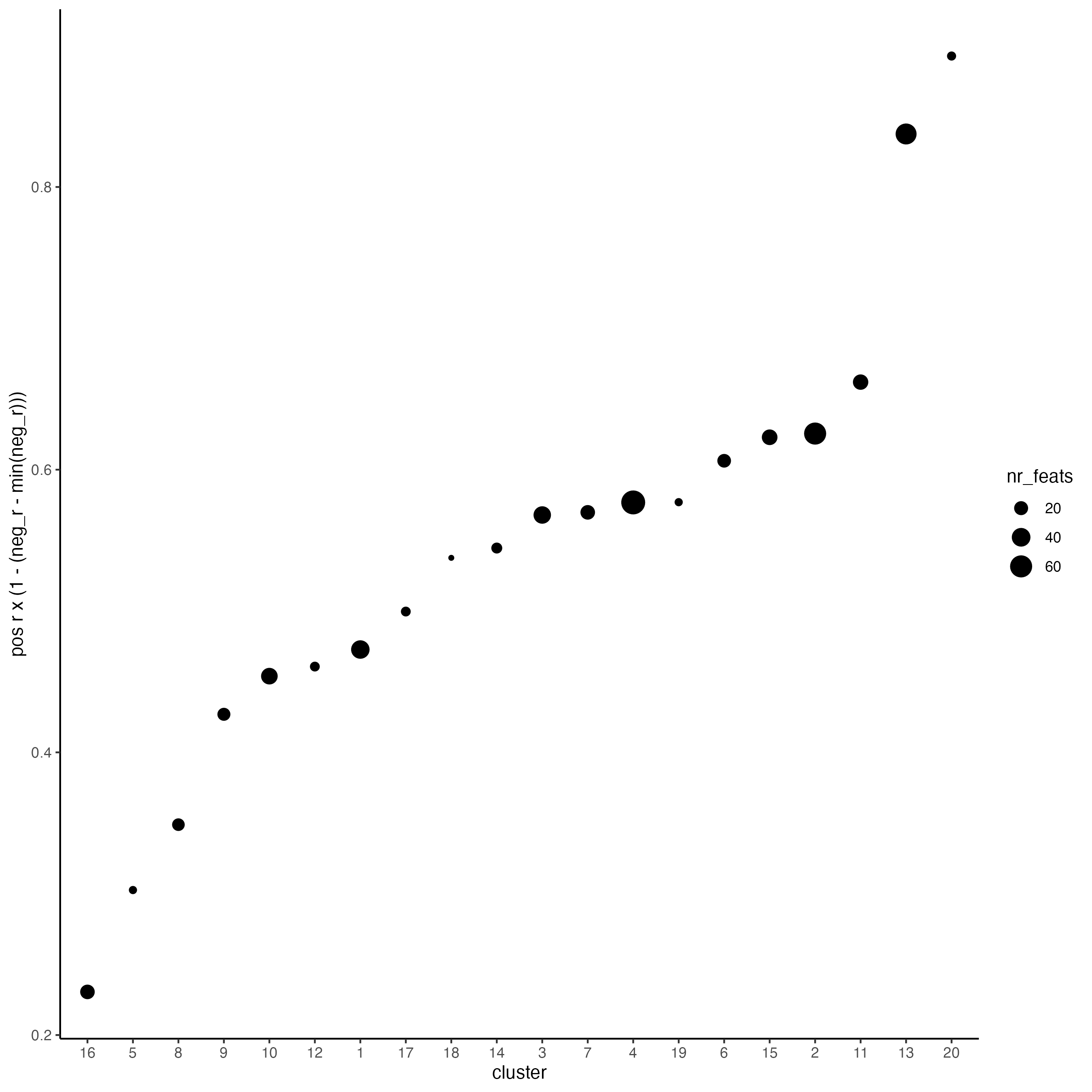
Figure 8.14: Ranking of spatial correlated groups. Size indicates the number spatial genes per group.
- Create the metagene enrichment score per co-expression cluster
cluster_genes_DT <- showSpatialCorFeats(spat_cor_netw_DT,
                                        use_clus_name = "spat_netw_clus",
                                        show_top_feats = 1)

cluster_genes <- cluster_genes_DT$clus
names(cluster_genes) <- cluster_genes_DT$feat_ID

visium_brain <- createMetafeats(visium_brain,
                                feat_clusters = cluster_genes,
                                name = "cluster_metagene")
Plot the spatial distribution of the metagene enrichment scores of each spatial co-expression cluster.
spatCellPlot(visium_brain,
             spat_enr_names = "cluster_metagene",
             cell_annotation_values = netw_ranks$clusters,
             point_size = 1,
             cow_n_col = 5)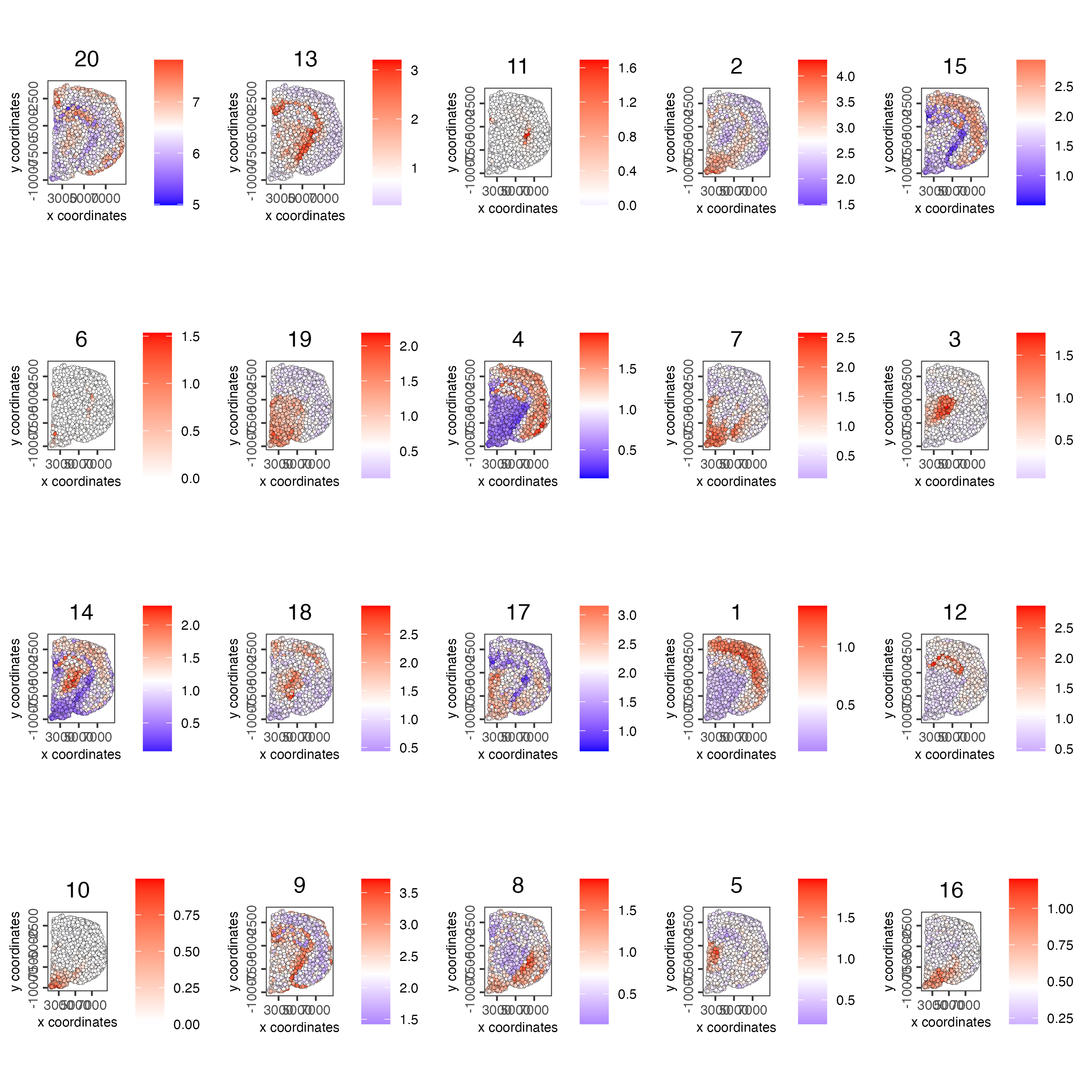
Figure 8.15: Spatial distribution of metagene enrichment scores per co-expression cluster.
8.5 Spatially informed clusters
- Get the top 30 genes per spatial co-expression cluster
coexpr_dt <- data.table::data.table(
  genes = names(spat_cor_netw_DT$cor_clusters$spat_netw_clus),
  cluster = spat_cor_netw_DT$cor_clusters$spat_netw_clus)

data.table::setorder(coexpr_dt, cluster)

top30_coexpr_dt <- coexpr_dt[, head(.SD, 30) , by = cluster]

spatial_genes <- top30_coexpr_dt$genes- Re-calculate the clustering
Use the spatial genes to calculate again the principal components, umap, network and clustering
visium_brain <- runPCA(gobject = visium_brain,
                       feats_to_use = spatial_genes,
                       name = "custom_pca")

visium_brain <- runUMAP(visium_brain,
                        dim_reduction_name = "custom_pca",
                        dimensions_to_use = 1:20,
                        name = "custom_umap")

visium_brain <- createNearestNetwork(gobject = visium_brain,
                                     dim_reduction_name = "custom_pca",
                                     dimensions_to_use = 1:20,
                                     k = 5,
                                     name = "custom_NN")

visium_brain <- doLeidenCluster(gobject = visium_brain,
                                network_name = "custom_NN",
                                resolution = 0.15,
                                n_iterations = 1000,
name = "custom_leiden")- Visualize
Plot the spatial distribution of the Leiden clusters calculated based on the spatial genes.
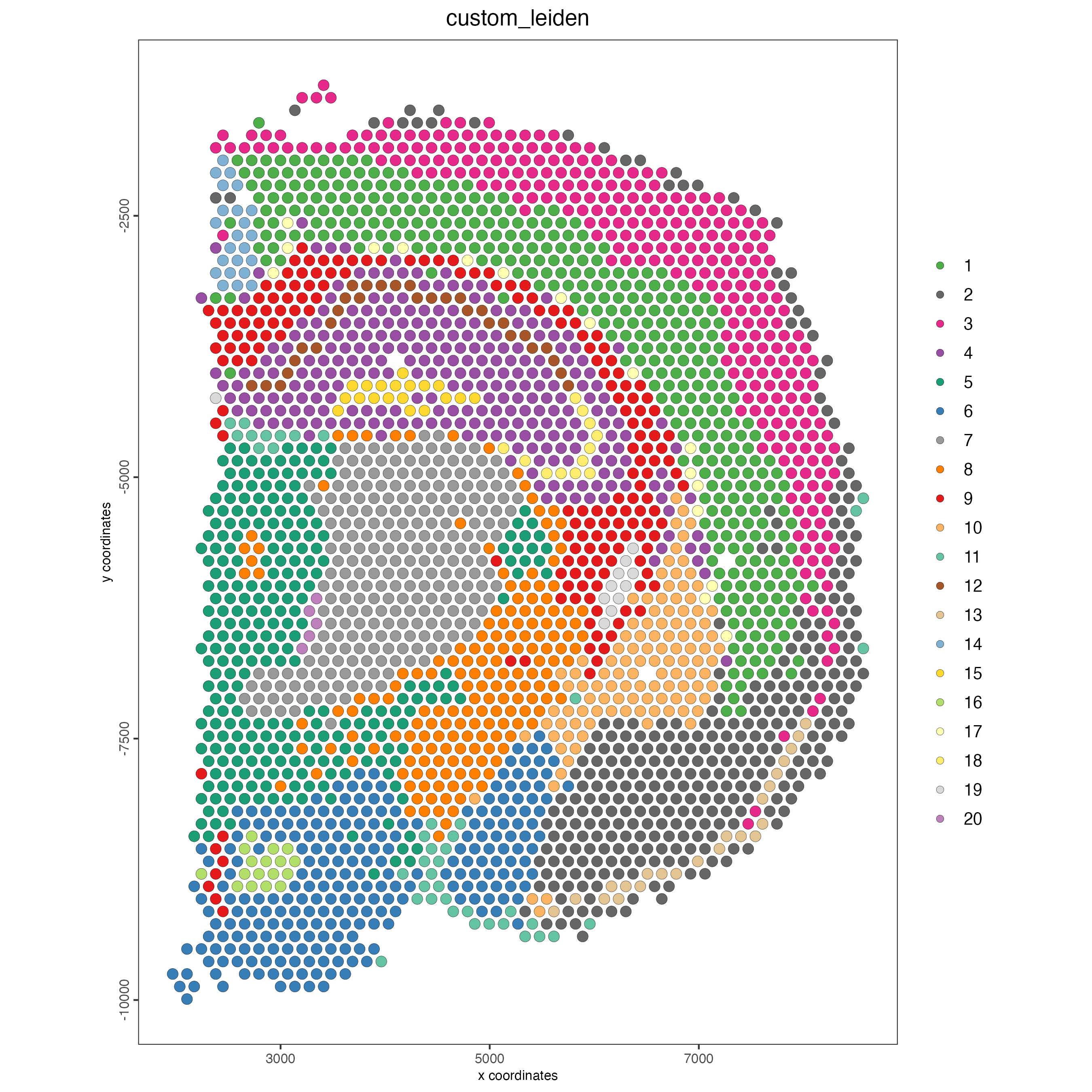
Figure 8.16: Spatial distribution of Leiden clusters calculated using spatial genes.
Plot the UMAP and color the spots using the Leiden clusters calculated based on the spatial genes.
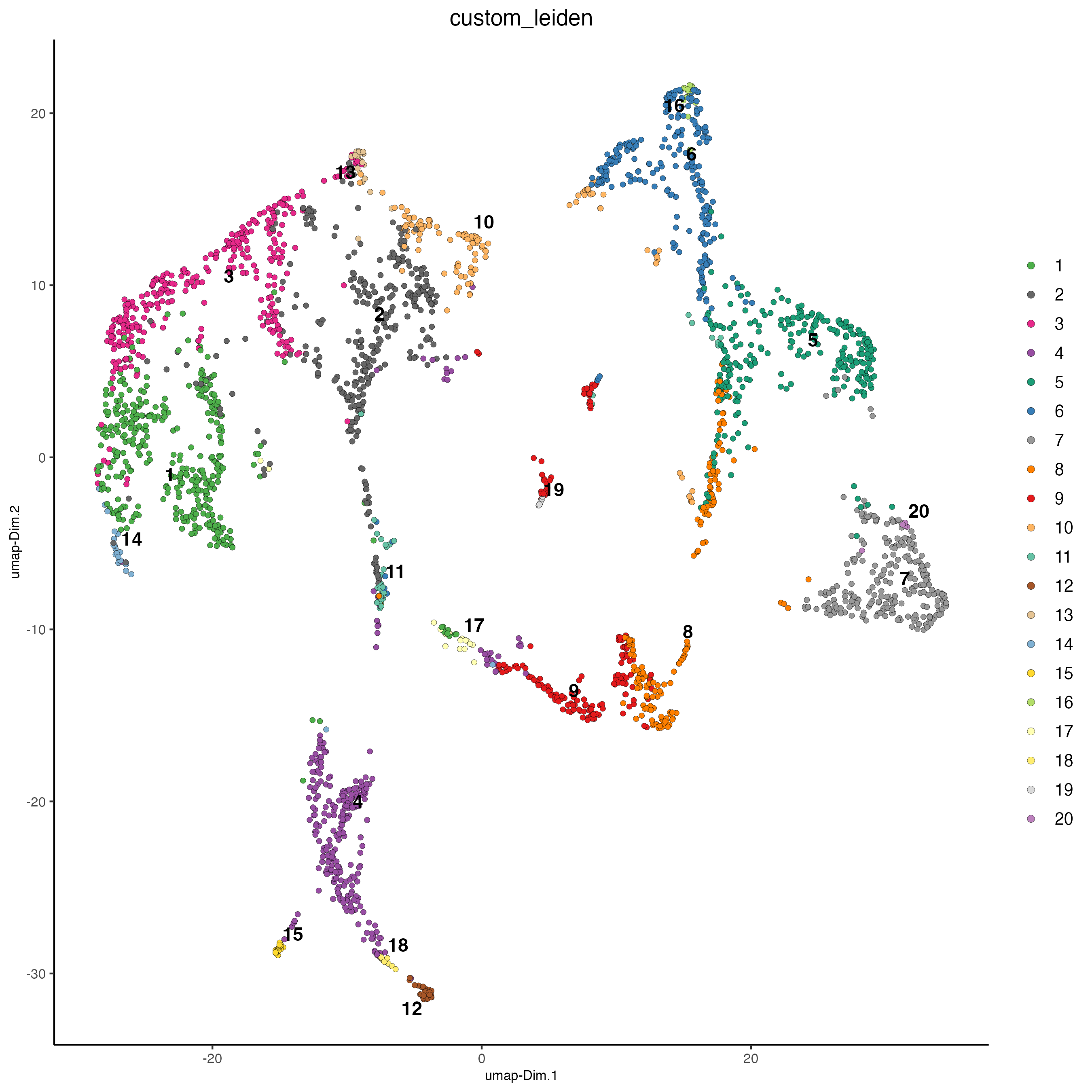
Figure 8.17: UMAP plot, colors indicate the Leiden clusters calculated using spatial genes.
8.6 Spatial domains HMRF
Hidden Markov Random Field (HMRF) models capture spatial dependencies and segment tissue regions based on shared and gene expression patterns.
- Do HMRF with different betas on top 30 genes per spatial co-expression module
This step may take several minutes to run.
HMRF_spatial_genes <- doHMRF(gobject = visium_brain,
                            expression_values = "scaled",
                            spatial_genes = spatial_genes,
                            k = 20,
                            spatial_network_name = "spatial_network",
                            betas = c(0, 10, 5),
                            output_folder = "11_HMRF/")
Add the HMRF results to the giotto object
visium_brain <- addHMRF(gobject = visium_brain,
                        HMRFoutput = HMRF_spatial_genes,
                        k = 20,
                        betas_to_add = c(0, 10, 20, 30, 40),
hmrf_name = "HMRF")- Visualize
Plot the spatial distribution of the HMRF domains.
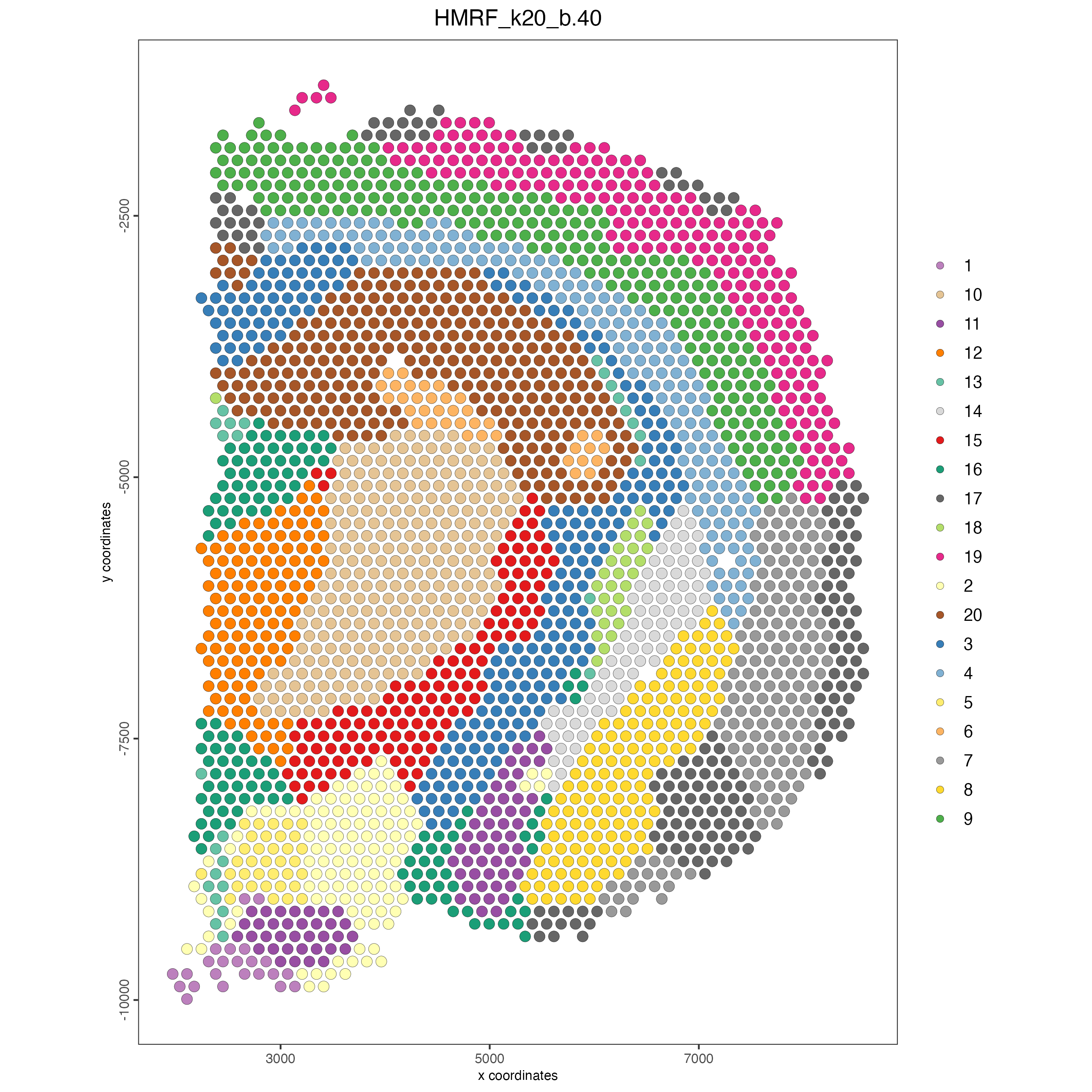
Figure 8.18: Spatial distribution of HMRF domains.
8.7 Interactive tools
We have integrated a shiny app in Giotto to interactively select regions of a spatial plot.
- Create a spatial plot
brain_spatPlot <- spatPlot2D(gobject = visium_brain,
                          cell_color = "leiden_clus",
                          show_image = FALSE,
                          return_plot = TRUE,
                          point_size = 1)

brain_spatPlot- Run the Shiny app
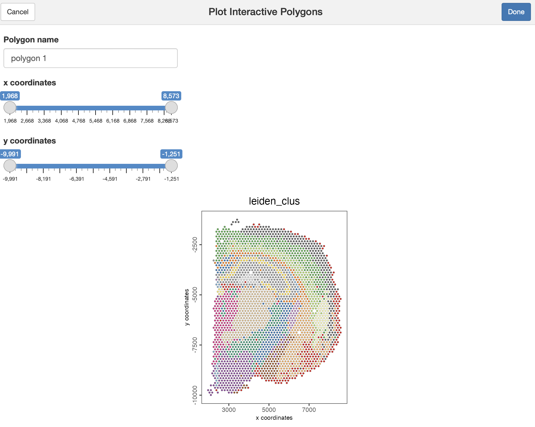
Figure 8.19: Shiny app using the visium brain sample.
- Select the regions of interest and save the coordinates
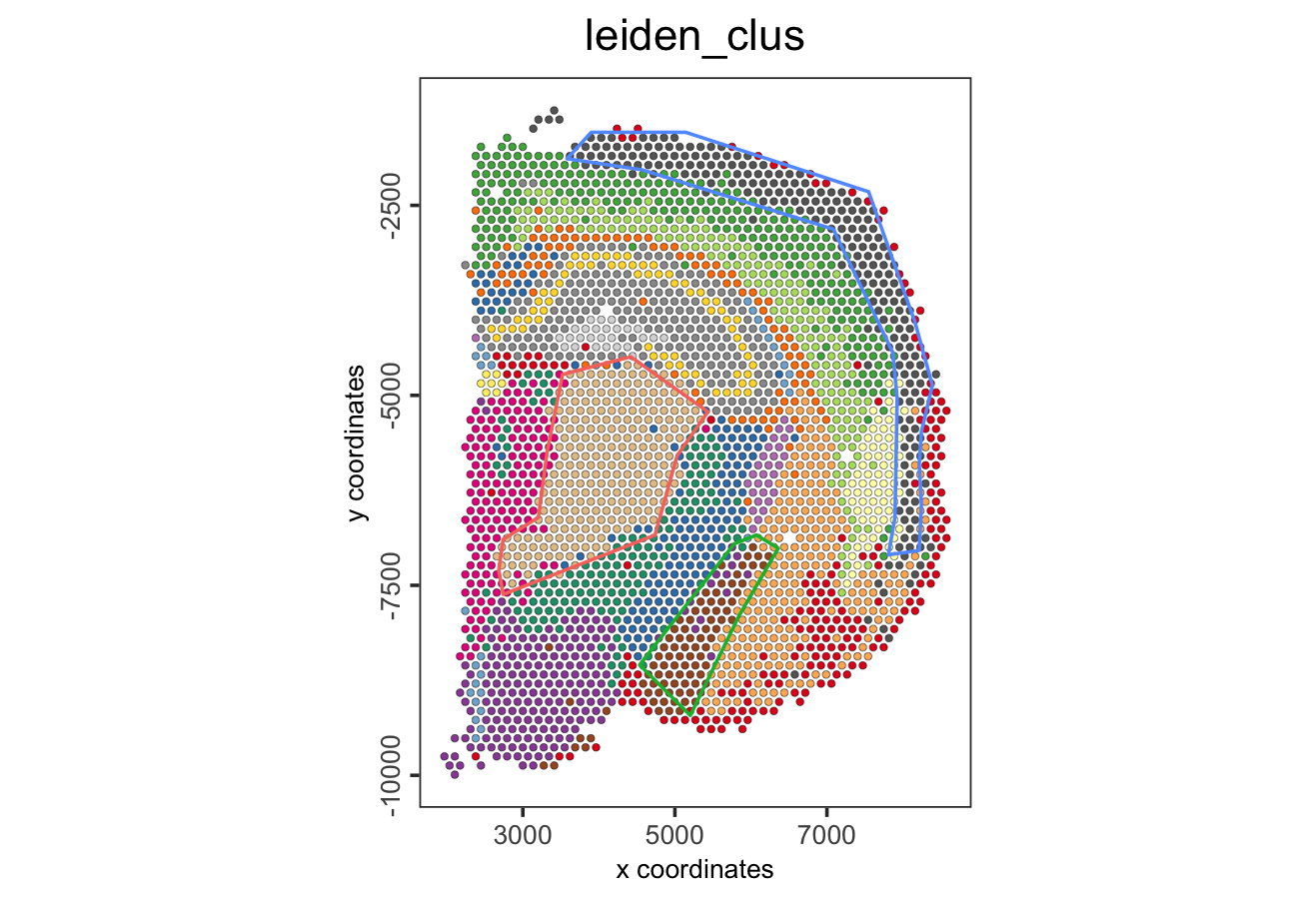
Figure 8.20: Polygons selected using the interactive Shiny app.
- Transform the data.table or data.frame with coordinates into a Giotto polygon object
giotto_polygons <- createGiottoPolygonsFromDfr(polygon_coordinates,
                                               name = "selections",
calc_centroids = TRUE)- Add the polygons to the Giotto object
- Add the corresponding polygon IDs to the cell metadata
- Extract the coordinates and IDs from cells located within one or multiple regions of interest.
If no polygon name is provided, the function will retrieve cells located within all polygons
- Compare the expression levels of some genes of interest between the selected regions
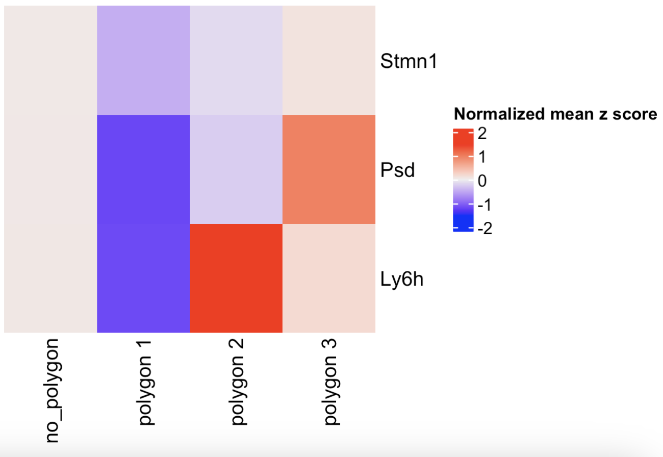
Figure 8.21: Heatmap showing the z-scores of three genes per selected polygon.
- Calculate the top genes expressed within each region, then provide the result to compare polygons
scran_results <- findMarkers_one_vs_all(
  visium_brain,
  spat_unit = "cell",
  feat_type = "rna",
  method = "scran",
  expression_values = "normalized",
  cluster_column = "selections",
  min_feats = 2)

top_genes <- scran_results[, head(.SD, 2), by = "cluster"]$feats

comparePolygonExpression(visium_brain,
                         selected_feats = top_genes)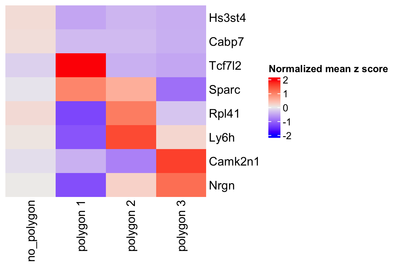
Figure 8.22: Heatmap showing the z-scores of top scran genes per selected polygon.
- Compare the abundance of cell types between the selected regions
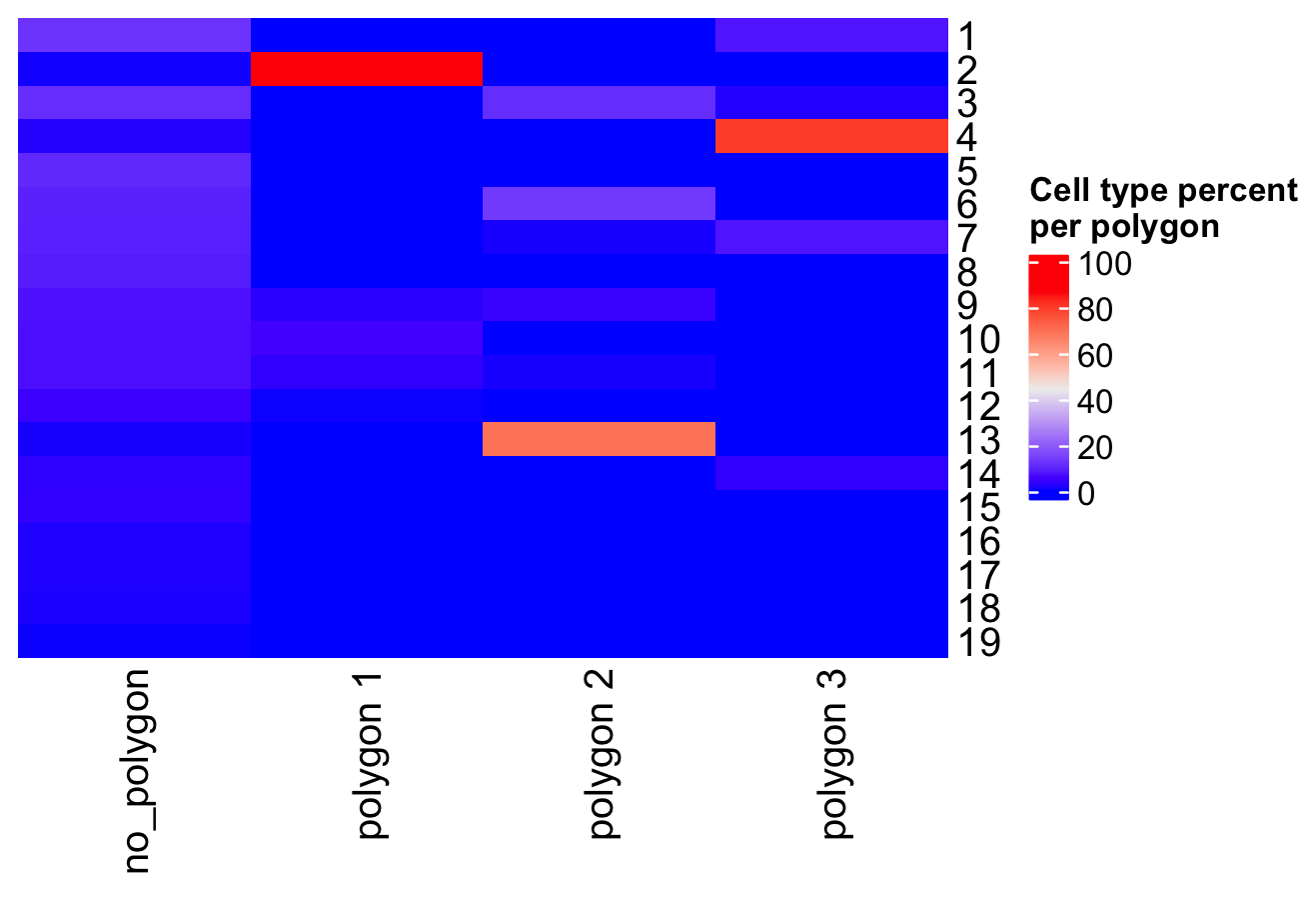
Figure 8.23: Heatmap showing the cell abundance per selected polygon.
- Use other columns within the cell metadata table to compare the cell type abundances
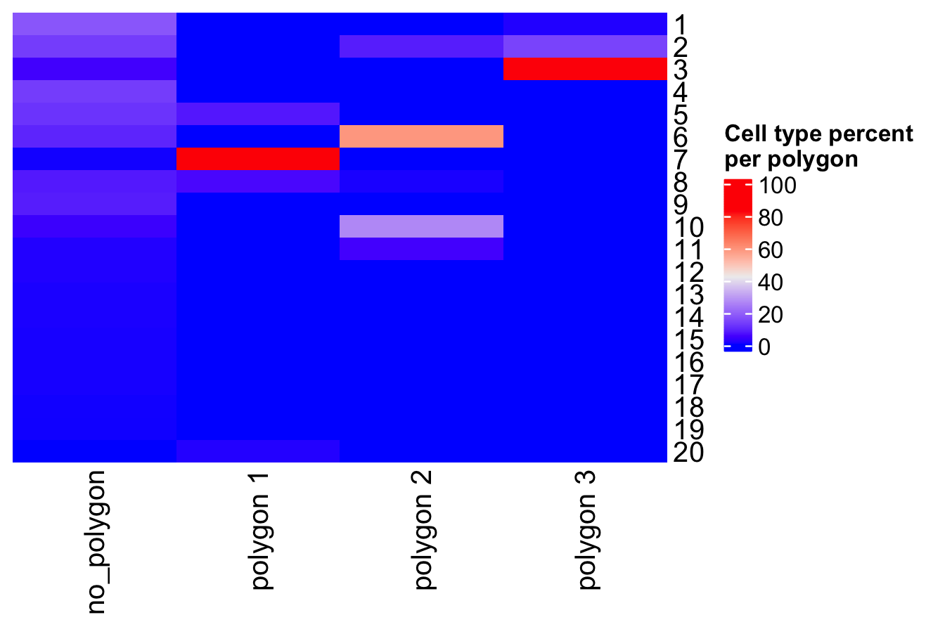
Figure 8.24: Heatmap showing the Leiden clusters abundance per selected polygon.
- Use the spatPlot arguments to isolate and plot each region.
spatPlot2D(visium_brain,
           cell_color = "leiden_clus",
           group_by = "selections",
           cow_n_col = 3,
           point_size = 2,
           show_legend = FALSE)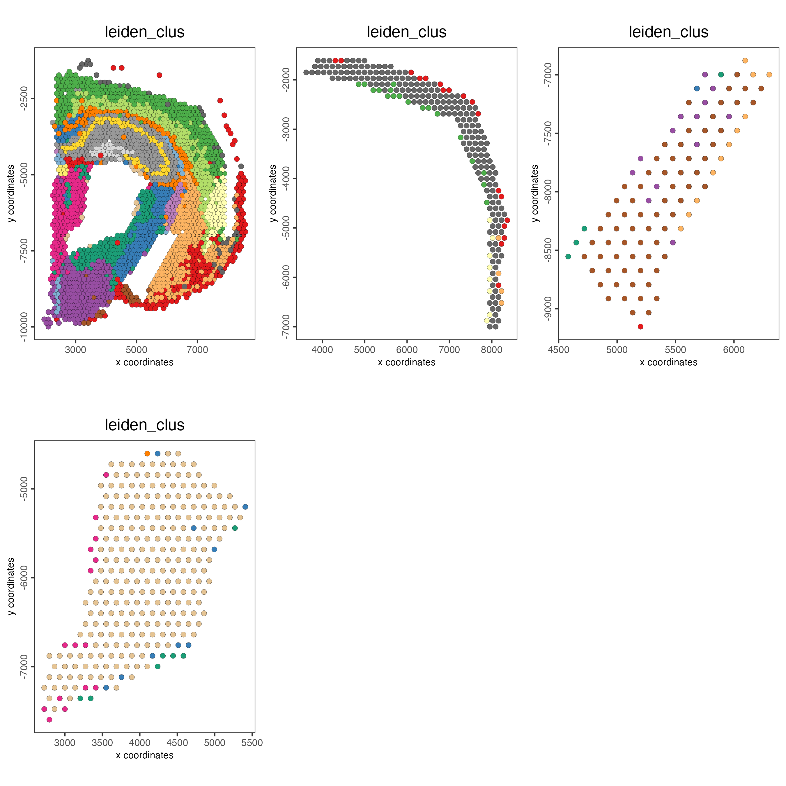
Figure 8.25: Spatial distribution of Leiden clusters across the selected polygons.
- Color each cell by cluster, cell type or expression level.
spatFeatPlot2D(visium_brain,
               expression_values = "scaled",
               group_by = "selections",
               feats = "Psd",
               point_size = 2)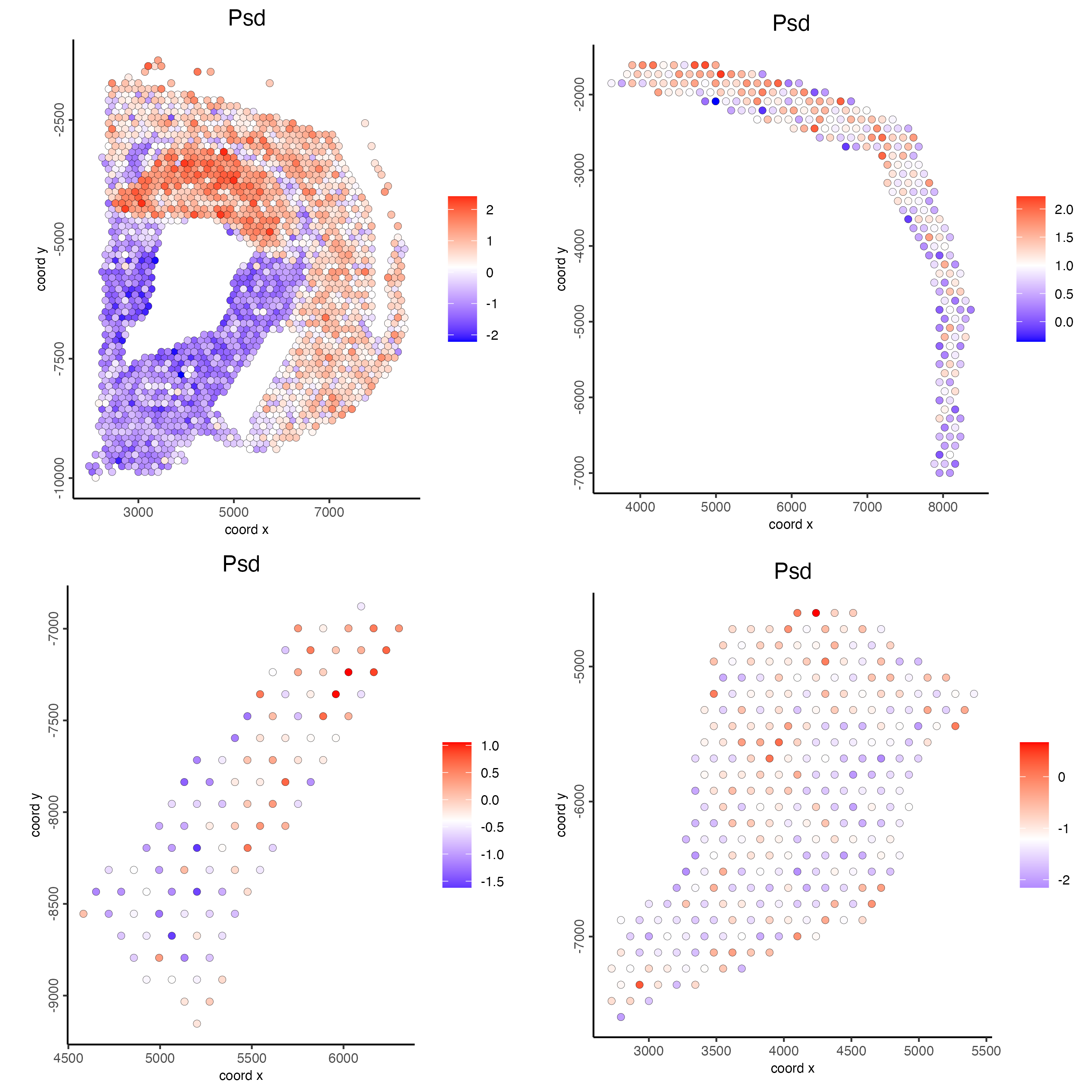
Figure 8.26: Spatial distribution of Psd scaled expression across the selected polygons.
- Plot again the polygons

Figure 8.27: Spatial location of selected polygons.
8.9 Session info
R version 4.4.1 (2024-06-14)
Platform: aarch64-apple-darwin20
Running under: macOS Sonoma 14.5

Matrix products: default
BLAS:   /System/Library/Frameworks/Accelerate.framework/Versions/A/Frameworks/vecLib.framework/Versions/A/libBLAS.dylib
LAPACK: /Library/Frameworks/R.framework/Versions/4.4-arm64/Resources/lib/libRlapack.dylib;  LAPACK version 3.12.0

locale:
[1] en_US.UTF-8/en_US.UTF-8/en_US.UTF-8/C/en_US.UTF-8/en_US.UTF-8

time zone: America/New_York
tzcode source: internal

attached base packages:
[1] stats     graphics  grDevices utils     datasets  methods   base

other attached packages:
[1] shiny_1.8.1.1     Giotto_4.1.0      GiottoClass_0.3.3

loaded via a namespace (and not attached):
  [1] later_1.3.2                 tibble_3.2.1
  [3] R.oo_1.26.0                 polyclip_1.10-7
  [5] lifecycle_1.0.4             edgeR_4.2.1
  [7] doParallel_1.0.17           lattice_0.22-6
  [9] MASS_7.3-61                 backports_1.5.0
 [11] magrittr_2.0.3              sass_0.4.9
 [13] limma_3.60.4                plotly_4.10.4
 [15] rmarkdown_2.27              jquerylib_0.1.4
 [17] yaml_2.3.9                  metapod_1.12.0
 [19] httpuv_1.6.15               sp_2.1-4
 [21] reticulate_1.38.0           cowplot_1.1.3
 [23] RColorBrewer_1.1-3          abind_1.4-5
 [25] zlibbioc_1.50.0             quadprog_1.5-8
 [27] GenomicRanges_1.56.1        purrr_1.0.2
 [29] R.utils_2.12.3              BiocGenerics_0.50.0
 [31] tweenr_2.0.3                circlize_0.4.16
 [33] GenomeInfoDbData_1.2.12     IRanges_2.38.1
 [35] S4Vectors_0.42.1            ggrepel_0.9.5
 [37] irlba_2.3.5.1               terra_1.7-78
 [39] dqrng_0.4.1                 DelayedMatrixStats_1.26.0
 [41] colorRamp2_0.1.0            codetools_0.2-20
 [43] DelayedArray_0.30.1         scuttle_1.14.0
 [45] ggforce_0.4.2               tidyselect_1.2.1
 [47] shape_1.4.6.1               UCSC.utils_1.0.0
 [49] farver_2.1.2                ScaledMatrix_1.12.0
 [51] matrixStats_1.3.0           stats4_4.4.1
 [53] GiottoData_0.2.12.0         jsonlite_1.8.8
 [55] GetoptLong_1.0.5            BiocNeighbors_1.22.0
 [57] progressr_0.14.0            iterators_1.0.14
 [59] systemfonts_1.1.0           foreach_1.5.2
 [61] dbscan_1.2-0                tools_4.4.1
 [63] ragg_1.3.2                  Rcpp_1.0.13
 [65] glue_1.7.0                  SparseArray_1.4.8
 [67] xfun_0.46                   MatrixGenerics_1.16.0
 [69] GenomeInfoDb_1.40.1         dplyr_1.1.4
 [71] withr_3.0.0                 fastmap_1.2.0
 [73] bluster_1.14.0              fansi_1.0.6
 [75] digest_0.6.36               rsvd_1.0.5
 [77] R6_2.5.1                    mime_0.12
 [79] textshaping_0.4.0           colorspace_2.1-0
 [81] scattermore_1.2             Cairo_1.6-2
 [83] gtools_3.9.5                R.methodsS3_1.8.2
 [85] utf8_1.2.4                  tidyr_1.3.1
 [87] generics_0.1.3              data.table_1.15.4
 [89] FNN_1.1.4                   httr_1.4.7
 [91] htmlwidgets_1.6.4           S4Arrays_1.4.1
 [93] scatterpie_0.2.3            uwot_0.2.2
 [95] pkgconfig_2.0.3             gtable_0.3.5
 [97] ComplexHeatmap_2.20.0       GiottoVisuals_0.2.4
 [99] SingleCellExperiment_1.26.0 XVector_0.44.0
[101] htmltools_0.5.8.1           bookdown_0.40
[103] clue_0.3-65                 scales_1.3.0
[105] Biobase_2.64.0              GiottoUtils_0.1.10
[107] png_0.1-8                   SpatialExperiment_1.14.0
[109] scran_1.32.0                ggfun_0.1.5
[111] knitr_1.48                  rstudioapi_0.16.0
[113] reshape2_1.4.4              rjson_0.2.21
[115] checkmate_2.3.1             cachem_1.1.0
[117] GlobalOptions_0.1.2         stringr_1.5.1
[119] parallel_4.4.1              miniUI_0.1.1.1
[121] RcppZiggurat_0.1.6          pillar_1.9.0
[123] grid_4.4.1                  vctrs_0.6.5
[125] promises_1.3.0              BiocSingular_1.20.0
[127] beachmat_2.20.0             xtable_1.8-4
[129] cluster_2.1.6               evaluate_0.24.0
[131] magick_2.8.4                cli_3.6.3
[133] locfit_1.5-9.10             compiler_4.4.1
[135] rlang_1.1.4                 crayon_1.5.3
[137] labeling_0.4.3              plyr_1.8.9
[139] stringi_1.8.4               viridisLite_0.4.2
[141] deldir_2.0-4                BiocParallel_1.38.0
[143] munsell_0.5.1               lazyeval_0.2.2
[145] Matrix_1.7-0                sparseMatrixStats_1.16.0
[147] ggplot2_3.5.1               statmod_1.5.0
[149] SummarizedExperiment_1.34.0 Rfast_2.1.0
[151] memoise_2.0.1               igraph_2.0.3
[153] bslib_0.7.0                 RcppParallel_5.1.8