10 Xenium
Jiaji George Chen
August 6th 2024
10.1 Introduction to spatial dataset
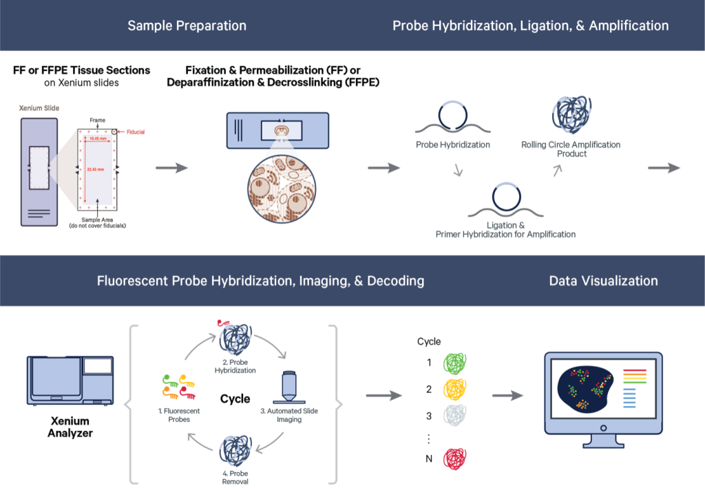
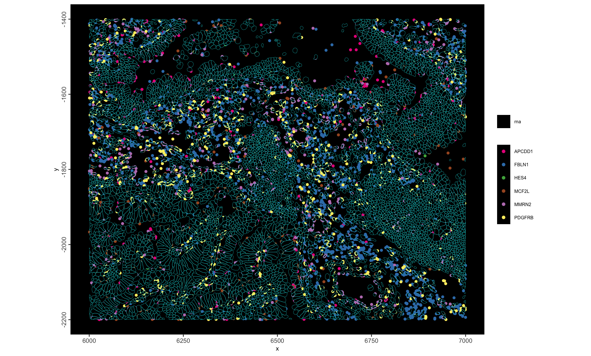
This is the 10X Xenium FFPE Human Lung Cancer dataset. Xenium captures individual transcript detections with a spatial resolution of 100s of nanometers, providing an extremely highly resolved subcellular spatial dataset. This particular dataset also showcases their recent multimodal cell segmentation outputs.
The Xenium Human Multi-Tissue and Cancer Panel (377) genes was used. The exported data is from their Xenium Onboard Analysis v2.0.0 pipeline.
The full data for this example can be found here: here
The relevant items are:
- Xenium Output Bundle (full)
- Supplemental: Post-Xenium H&E image (OME-TIFF)
- Supplemental: H&E Image Alignment File (CSV)
Additional package requirements
When working with this data and trying to open the parquet files, you will need arrow built with ZTSD support. See the datasets & packages section for specific install instructions.
10.1.1 Output directory structure
    ├── analysis.tar.gz
    ├── analysis.zarr.zip
    ├── analysis_summary.html
    ├── aux_outputs.tar.gz
    ├── transcripts.csv.gz
    ├── transcripts.parquet
    ├── transcripts.zarr.zip
    ├── cell_boundaries.csv.gz
    ├── cell_boundaries.parquet
    ├── nucleus_boundaries.csv.gz
    ├── nucleus_boundaries.parquet
    ├── cell_feature_matrix.tar.gz
    ├── cell_feature_matrix
    │   ├── barcodes.tsv.gz
    │   ├── features.tsv.gz
    │   └── matrix.mtx.gz
    ├── cell_feature_matrix.h5
    ├── cell_feature_matrix.zarr.zip
    ├── cells.csv.gz
    ├── cells.parquet
    ├── cells.zarr.zip
    ├── experiment.xenium
    ├── gene_panel.json
    ├── metrics_summary.csv
    ├── morphology.ome.tif
    ├── morphology_focus
    │   ├── morphology_focus_0000.ome.tif
    │   ├── morphology_focus_0001.ome.tif
    │   ├── morphology_focus_0002.ome.tif
    │   ├── morphology_focus_0003.ome.tif
    ├── Xenium_V1_humanLung_Cancer_FFPE_he_image.ome.tif
    └── Xenium_V1_humanLung_Cancer_FFPE_he_imagealignment.csv
The above directory structuring and naming is characteristic of Xenium v2.0 pipeline outputs. The only items that may not be exactly the same across all outputs are the morphology focus directory and the naming of the aligned image items.
For the morphology focus images, you may have fewer images if the experiment did not include the multimodal cell segmentation. As for the aligned images, this is usually done after the Xenium experiment concludes and is added on using Xenium Explorer. Naming and location of the aligned image (he_image.ome.tif) and associated alignment info he_imagealignment.csv are entirely up to the user.
10.1.2 Mini Xenium Dataset
library(Giotto)

# set up paths
data_path <- "data/02_session3"
save_dir <- "results/02_session3"
dir.create(save_dir, recursive = TRUE)

# download the mini dataset and untar
options("timeout" = Inf)
download.file(
    url = "https://zenodo.org/records/13207308/files/workshop_xenium.zip?download=1",
    destfile = file.path(save_dir, "workshop_xenium.zip")
)
# untar the downloaded data
untar(tarfile = file.path(save_dir, "workshop_xenium.zip"),
      exdir = data_path)
In order to speed up the steps of the workshop and make it locally runnable, we provide a subset of the full dataset.
- Full: -16.039, 12342.984, -3511.515, -294.455 (xmin, xmax, ymin, ymax)
- Mini: 6000,    7000,      -2200,     -1400    (xmin, xmax, ymin, ymax)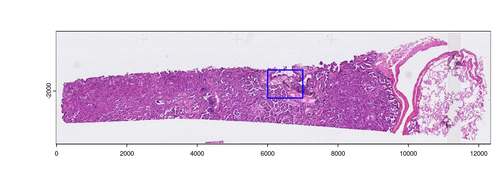
Figure 10.1: Shown is the H&E aligned to the Xenium dataset with micron scaling. The blue bounds mark out the area provided as a mini dataset
10.2 Data preparation
10.2.1 Image conversion (may change)
First is actually dealing with the image formats. Xenium generates ome.tif images which Giotto is currently not fully compatible with. So we convert them to normal tif images using ometif_to_tif() which works through the python tifffile package.
The image files can then be loaded in downstream steps.
These commented out steps are not needed for today since the mini dataset provides .tif images that have already been spatially aligned and converted. However, the code needed to do this is provided below.
# image_paths <- list.files(
#   data_path, pattern = "morphology_focus|he_image.ome",
#   recursive = TRUE, full.names = TRUE
# )
ometif_to_tif() output_dir can be specified, but by default, it writes to a new subdirectory called tif_exports underneath the source image”s directory.
Keep in mind that where the exported tifs get exported to should be where downstream image reading functions should point to. The code run today is with the filepaths that the mini dataset has.
We are also working on a method of directly accessing the ome.tifs for better compatibility in the future.
10.3 Convenience function
Giotto has flexible methods for working with the Xenium outputs. The createGiottoXeniumObject() will generate a giotto object in a single step when provided the output directory.
The default behavior is to load:
- transcripts information
- cell and nucleus boundaries
- feature metadata (gene_panel.json)
For the full dataset (HPC): time: 1-2min | memory: 24GBC
?createGiottoXeniumObject

g <- createGiottoXeniumObject(xenium_dir = data_path)

# set instructions for save directory and to save the plots to disk
instructions(g, "save_dir") <- save_dir
instructions(g, "save_plot") <- TRUE
There are a lot of other parameters for additional or alternative items you can load. The next subsections will explain a couple of them.
10.3.1 Specific filepaths
expression_path = ,
cell_metadata_path = ,
transcript_path = ,
bounds_path = ,
gene_panel_json_path = ,
The convenience function auto-detects filepaths based on the Xenium directory path and the preferred file formats
.parquetfor tabular (vs.csv).h5for matrix over other formats when available (vs.mtx).zarris currently not supported.
When you need to use a different file format or something is not in the expected output structure, you can supply a specific filepath to the convenience function using these parameters.
10.3.2 Quality value
qv_threshold = 20 # defaultThe Quality Value is a Phred-based 0-40 value that 10X provides for every detection in their transcripts output. Higher values mean higher confidence in the decoded transcript identity. By default 10X uses a cutoff of QV = 20 for transcripts to use downstream.
_*setting a value other than 20 will make the loaded dataset different from the 10X-provided expression matrix and cell metadata._
QV Calculation
- Raw Q-score based on how likely it is that an observed code is to be the codeword that it gets mapped to vs less likely codeword.
- Adjustment of raw Q-score by binning the transcripts by Q-value then adjusting the exact Q per bin based on proportion of Negative Control Codewords detected within.
10.3.3 Transcript type splitting
feat_type =  c(
    "rna",
    "NegControlProbe",
    "UnassignedCodeword",
    "NegControlCodeword"
),
split_keyword = list(
    c("NegControlProbe"),
    c("UnassignedCodeword"),
    c("NegControlCodeword)"
)
There are 4 types of transcript detections that 10X reports with their v2.0 pipeline:
- Gene expression - This is the rna gene detections.
- Negative Control Codeword - (QC) Codewords that do not map to genes, but are in the codebook. Used to determine specificity of decoding algorithm.
- Negative Control Probe - (QC) Probes in panel but target non-biological sequences. Used to determine specificity of assay.
- Unassigned Codeword - (QC) Codewords that should not be used in the current panel.
With V3 on their Xenium prime outputs, there is additionally:
- Genomic Control Codeword (QC) Probes for intergenic genomic DNA instead of transcripts.
The main thing to watch out for is that the other probe types should be separated out from the the Gene expression or rna feature type.
How to deal with these different types of detections is easily adjustable. With the feat_type param you declare which categories/feat_types you want to split transcript detections into. Then with split_keyword, you provide a list of character vectors containing grep() terms to search for.
Note that there are 4 feat_types declared in this set of defaults, but 3 items passed to split_keyword. Any transcripts not matched by items in split_keyword, get categorized as the first provided feat_type (“rna”).
10.4 Piecewise loading
Giotto also provides the importXenium() import utility that allows independent creation of compatible Giotto subobjects for more flexibility.
Giotto <XeniumReader>
dir       : data/02_session3/
qv_cutoff : 20
filetype  : transcripts -- parquet
boundaries  -- parquet
expression  -- h5
cell_meta   -- parquet
funs      : load_transcripts()
load_polys()
load_cellmeta()
load_featmeta()
load_expression()
load_image()
load_aligned_image()
create_gobject()
10.4.1 Load giottoPoints transcripts
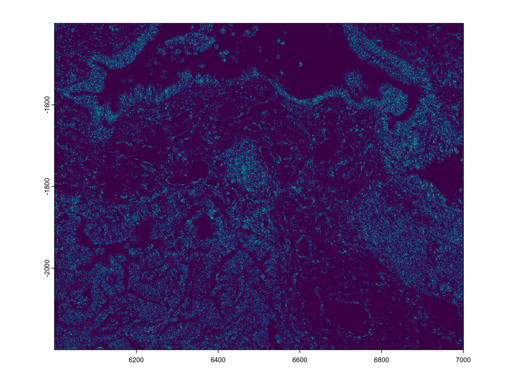
Figure 10.3: plot of Gene expression (rna) density
An object of class giottoPoints
feat_type : "rna"
Feature Information:
class       : SpatVector
geometry    : points
dimensions  : 479097, 10  (geometries, attributes)
extent      : 6000.001, 7000, -2200, -1400.012  (xmin, xmax, ymin, ymax)
coord. ref. :
names       : feat_ID   transcript_id    cell_id overlaps_nucleus z_location    qv fov_name
type        :   <chr>           <chr>      <chr>            <int>      <num> <num>    <chr>
values      :   FBLN1 281487861612869 mcnjadoe-1                0      19.32    40      B11
PDGFRB 281487861612872 mcnjbidl-1                1      18.75    40      B11
PDGFRB 281487861612873 mcnjbidl-1                1      18.74    40      B11
nucleus_distance codeword_index feat_ID_uniq
<num>          <int>        <int>
0            334            1
0            289            2
0 289 310.4.2 (optional) Loading pre-aggregated data
Giotto can spatially aggregate the transcripts information based on a provided set of boundaries information, however 10X also provides a pre-aggregated set of cell by feature information and metadata. These values may be slightly different from those calculated by Giotto”s pipeline, and are not loaded by default.
Some care needs to be taken when loading this information:
- The
feat_typeof the loaded expression information should be matched to the usedfeat_typeparameters passed to the convenience function. - The
qv_thresholdused must be 20 since the 10X outputs are based on that cutoff.
x$filetype$expression <- "mtx" # change to mtx instead of .h5 which is not in the mini dataset

ex <- x$load_expression()
featType(ex)
[1] "rna" "Negative Control Probe" "Negative Control Codeword"
[4] "Unassigned Codeword" The feature types here do not match what we established for the transcripts, so we can just change them.
Another reason for changing them here is just because the default names have ’ ’ characters which are difficult to work with.
An object of class giotto
>Active spat_unit:  cell
>Active feat_type:  rna
[SUBCELLULAR INFO]
polygons      : cell nucleus
features      : rna NegControlProbe UnassignedCodeword NegControlCodeword
[AGGREGATE INFO]
spatial locations ----------------
[cell] raw
[nucleus] rawfeatType(ex[[2]]) <- c("NegControlProbe")
featType(ex[[3]]) <- c("NegControlCodeword")
featType(ex[[4]]) <- c("UnassignedCodeword")Then we can just append them to the Giotto object.
Here we set up a second object called g2 since we will be using Giotto’s own aggregation method to generate the expression matrix later.
g2 <- g
# append the expression info
g2 <- setGiotto(g2, ex)

# load cell metadata
cx <- x$load_cellmeta()
g2 <- setGiotto(g2, cx)

force(g2)
An object of class giotto
>Active spat_unit: cell
>Active feat_type: rna
[SUBCELLULAR INFO]
polygons : cell nucleus
features : rna NegControlProbe UnassignedCodeword NegControlCodeword
[AGGREGATE INFO]
expression -----------------------
[cell][rna] raw
[cell][NegControlProbe] raw
[cell][NegControlCodeword] raw
[cell][UnassignedCodeword] raw
spatial locations ----------------
[cell] raw
[nucleus] rawspatInSituPlotPoints(g2,
# polygon shading params
polygon_fill = "cell_area",
polygon_fill_as_factor = FALSE,
polygon_fill_gradient_style = "sequential",
# polygon line params
polygon_color = "grey",
polygon_line_size = 0.1
)
spatInSituPlotPoints(g2,
# polygon shading params
polygon_fill = "transcript_counts",
polygon_fill_as_factor = FALSE,
polygon_fill_gradient_style = "sequential",
# polygon line params
polygon_color = "grey",
polygon_line_size = 0.1
)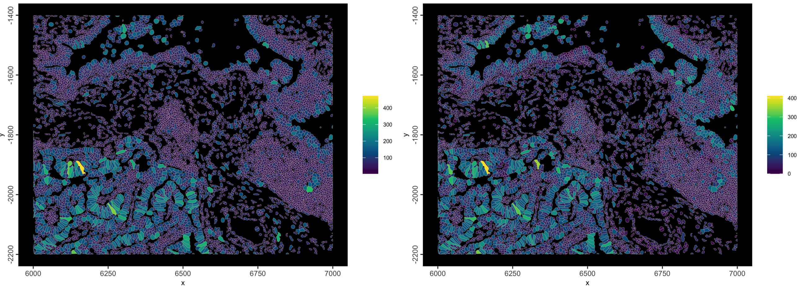
Figure 10.4: Example plot using 10X metadata. Left is cell_area, right is transcript_counts
10.5 Xenium Images
Xenium outputs have several image outputs. For this dataset:
morphology.ome.tifis a z-stacked image of the DAPI staining, with z levels separated as pages within theome.tif. In this dataset, only pages 6 and 7 are really in focus.morphology_focusis a folder containing single-channel image(s), but with the original z information collapsed into a single in-focus layer. For all datasets, image 0000 will be DAPI staining, but if you have additional stains, such as the multimodal segmentation, they will also be here. These are the recommended immunofluorescence staining images to import.Xenium_V1_humanLung_Cancer_FFPE_he_image.ome.tifis an added on (in this case H&E) image with manual affine registration.
10.5.1 Image metadata
The morphology_focus directory may contain multiple images, but to know more information, we have to check the ome.tif xml metadata. With a normal dataset, you can use:
`GiottoClass::ometif_metadata([filepath], node = "Channel")`on one of the morphology_focus images, but since the mini dataset images are pre-processed, there is only an exported .xml to explore. The output of the code chunk below is the same as that from calling ometif_metadata() and looking for the Channel node.
img_xml_path <- file.path(data_path, "morphology_focus", "morphology_focus_0000.xml")
omemeta <- xml2::read_xml(img_xml_path)
res <- xml2::xml_find_all(omemeta, "//d1:Channel", ns = xml2::xml_ns(omemeta))
res <- Reduce(rbind, xml2::xml_attrs(res))
rownames(res) <- NULL
res <- as.data.frame(res)
force(res)
ID Name SamplesPerPixel
1 Channel:0 DAPI 1
2 Channel:1 18S 1
3 Channel:2 ATP1A1/CD45/E-Cadherin 1
4 Channel:3 alphaSMA/Vimentin 110.5.2 Image loading
morphology_focus images need to be scaled by the micron scaling factor. Aligned images need to first be affine transformed then scaled. The micron scaling factor can be found in the json-like experiment.xenium file under pixel_size (0.2125 for this dataset).
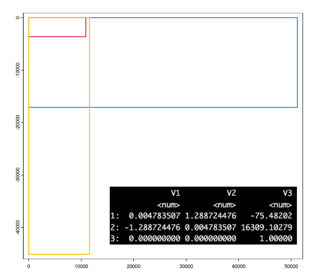
Figure 10.5: Spatial extent/bounds of transcripts (red), immunofluorescence morphology focus images (blue), H&E aligned image (gold). Lower right shows the affine matrix for aligning the H&E
These transforms are normally done automatically when using:
# convenience function params
load_images = list(
    img1 = "[img_path1.tif]",
    img2 = "[img_path2.tif]",
    img3 = "..."
),
load_aligned_images = list(
    aligned_img = c(
        "[path to image.tif]",
        "[path to magealignment.csv]"
    )
)

# importer params
x$load_image(path = "[img_path1.tif]", name = "img1")
x$load_image(path = "[img_path2.tif]", name = "img2")
...
x$load_aligned_image(
    path = "[path to image.tif]",
    imagealignment_path = "[path to magealignment.csv]",
    name = "aligned_img"
)
Specifically for the aligned image, there is also read10xAffineImage() which has similar parameters, but also asks for the micron scaling factor.
But for the mini dataset, the images are pre-processed and can be directly added.
img_paths <- c(
    sprintf("data/02_session3/morphology_focus/morphology_focus_%04d.tif", 0:3),
    "data/02_session3/he_mini.tif"
)

img_list <- createGiottoLargeImageList(
    img_paths,
    # naming is based on the channel metadata above
    names = c("DAPI", "18S", "ATP1A1/CD45/E-Cadherin", "alphaSMA/Vimentin", "HE"),
    use_rast_ext = TRUE,
    verbose = FALSE
)

# make some images brighter
img_list[[1]]@max_window <- 5000
img_list[[2]]@max_window <- 5000
img_list[[3]]@max_window <- 5000

# append images to gobject
g <- setGiotto(g, img_list)
# example plots
spatInSituPlotPoints(g,
show_image = TRUE,
image_name = "HE",
polygon_feat_type = "cell",
polygon_color = "cyan",
polygon_line_size = 0.1,
polygon_alpha = 0
)spatInSituPlotPoints(g,
show_image = TRUE,
image_name = "DAPI",
polygon_feat_type = "nucleus",
polygon_color = "cyan",
polygon_line_size = 0.1,
polygon_alpha = 0
)spatInSituPlotPoints(g,
show_image = TRUE,
image_name = "18S",
polygon_feat_type = "cell",
polygon_color = "cyan",
polygon_line_size = 0.1,
polygon_alpha = 0
)spatInSituPlotPoints(g,
show_image = TRUE,
image_name = "ATP1A1/CD45/E-Cadherin",
polygon_feat_type = "nucleus",
polygon_color = "cyan",
polygon_line_size = 0.1,
polygon_alpha = 0
)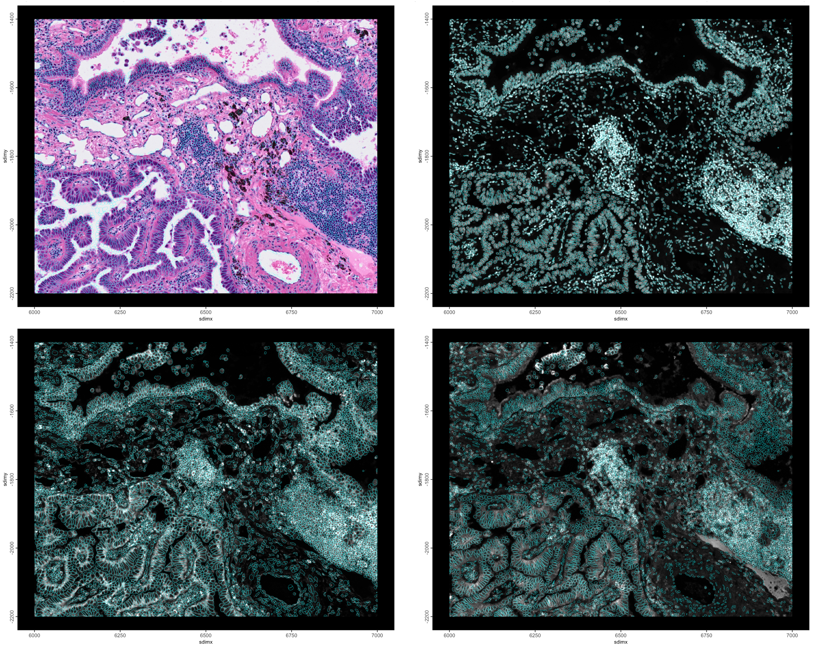
Figure 10.6: H&E and Cell polys (top left), DAPI and nuclear polys (top right), 18S and cell polys (lower left), ATP1A1/CD45/E-Cadherin and nuclear polys (lower right)
10.6 Spatial aggregation
First calculate the feat_info “rna” transcripts overlapped by the spatial_info “cell” polygons with calculateOverlap(). Then, the overlaps information (relationships between points and polygons that overlap them) gets converted into a count matrix with overlapToMatrix().
10.7 Aggregate analyses workflow
10.7.1 Transcripts per cell
g <- addStatistics(g) # this is going to fail because it looks for normalized

g <- addStatistics(g, expression_values = "raw")
cell_stats <- pDataDT(g)
ggplot2::ggplot(cell_stats, ggplot2::aes(total_expr)) +
ggplot2::geom_histogram(binwidth = 5)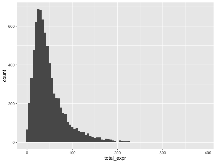
Figure 10.7: Histogram of detections per cell
10.7.2 Filtering
# very permissive filtering. Mainly for removing 0 values
g <- filterGiotto(g,
    expression_threshold = 1,
    feat_det_in_min_cells = 1,
    min_det_feats_per_cell = 5
)
Feature type: rna
Number of cells removed: 143 out of 7655
Number of feats removed: 0 out of 377 10.7.3 Normalization
g <- normalizeGiotto(g)
# overwrite original results with those for normalized values
g <- addStatistics(g)spatInSituPlotPoints(g,
polygon_fill = "nr_feats",
polygon_fill_gradient_style = "sequential",
polygon_fill_as_factor = FALSE
)spatInSituPlotPoints(g,
polygon_fill = "total_expr",
polygon_fill_gradient_style = "sequential",
polygon_fill_as_factor = FALSE
)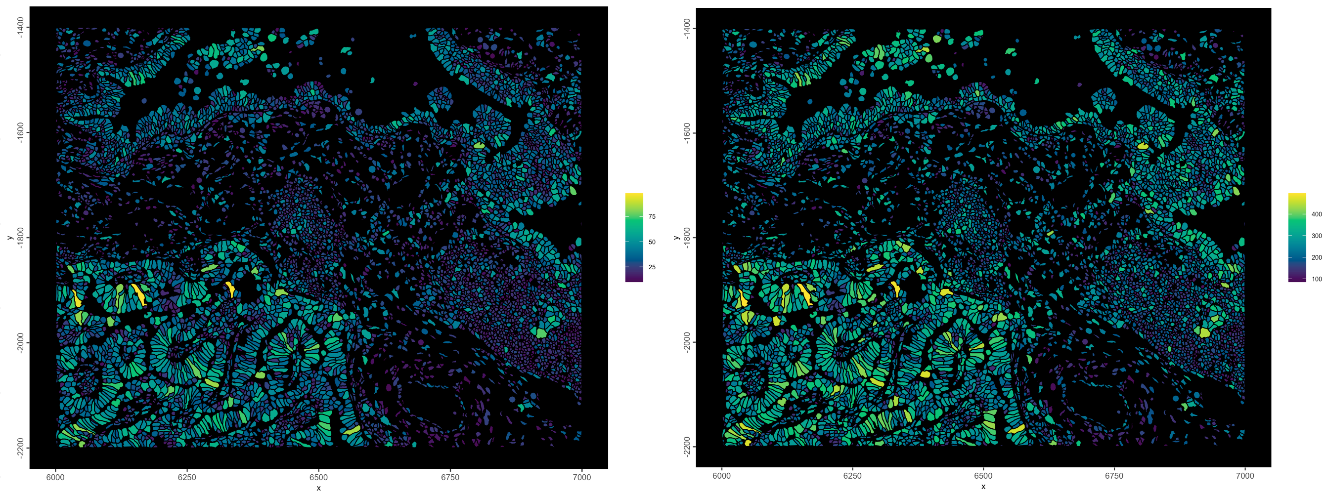
Figure 10.8: nr_feats - Number of different gene species detected per cell (left), total_expr - total detections per cell (right)
When there are a lot of features, we would also select only the interesting highly variable features so that downstream dimension reduction has more meaningful separation. Here we skip HVF detection since there are only 377 genes.
10.7.4 Dimension Reduction
Dimensional reduction of expression space to visualize expressional differences between cells and help with clustering.
g <- runPCA(g, feats_to_use = NULL)
# feats_to_use = NULL since there are no HVFs calculated. Use all genes.

screePlot(g, ncp = 30)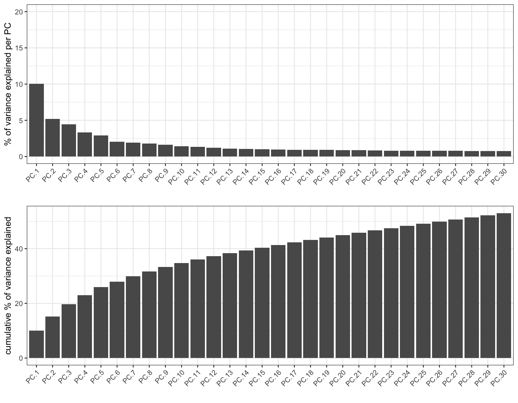
Figure 10.9: Plot of variance explained in the first 30 out of 100 principle components calculated
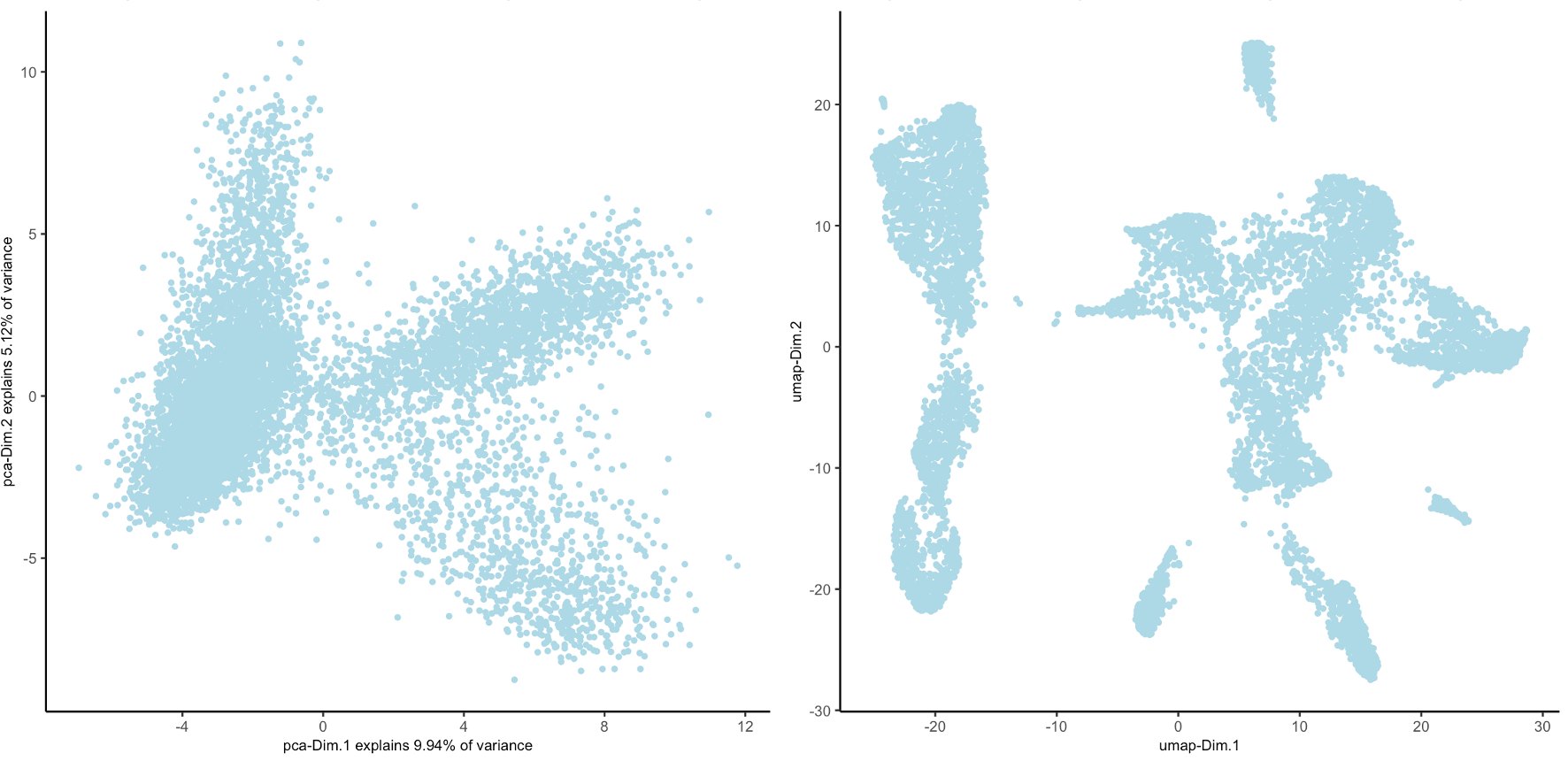
Figure 10.10: PCA plot showing the first 2 PCs (left), UMAP generated from first 15 PCs (right)
10.7.5 Clustering
g <- createNearestNetwork(g,
    dimensions_to_use = seq(15),
    k = 40
)

# takes roughly 1 min to run
g <- doLeidenCluster(g)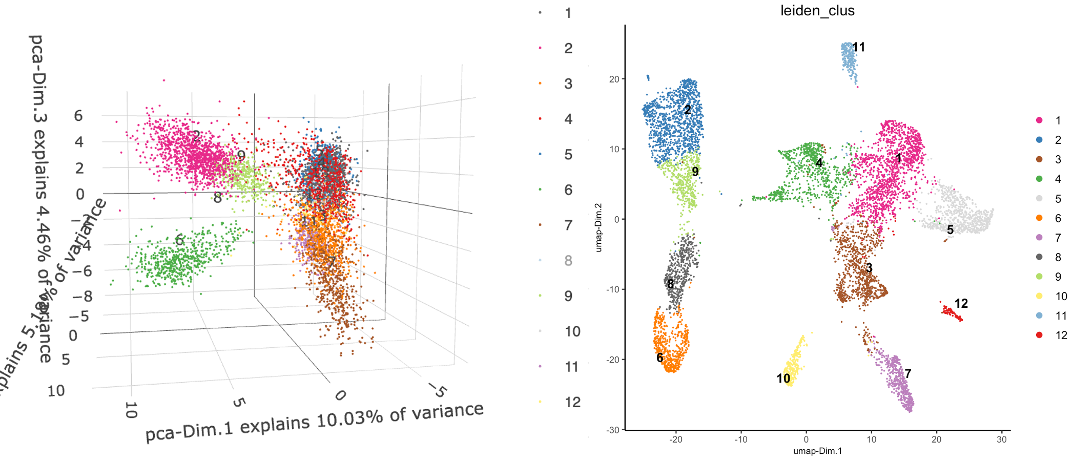
Figure 10.11: 3D plot showing first PCs with leiden clustering annotations (left), UMAP plot showing leiden clustering results (right)
spatInSituPlotPoints(g,
    polygon_fill = "leiden_clus",
    polygon_fill_as_factor = TRUE,
    polygon_alpha = 1,
    show_image = TRUE,
    image_name = "HE"
)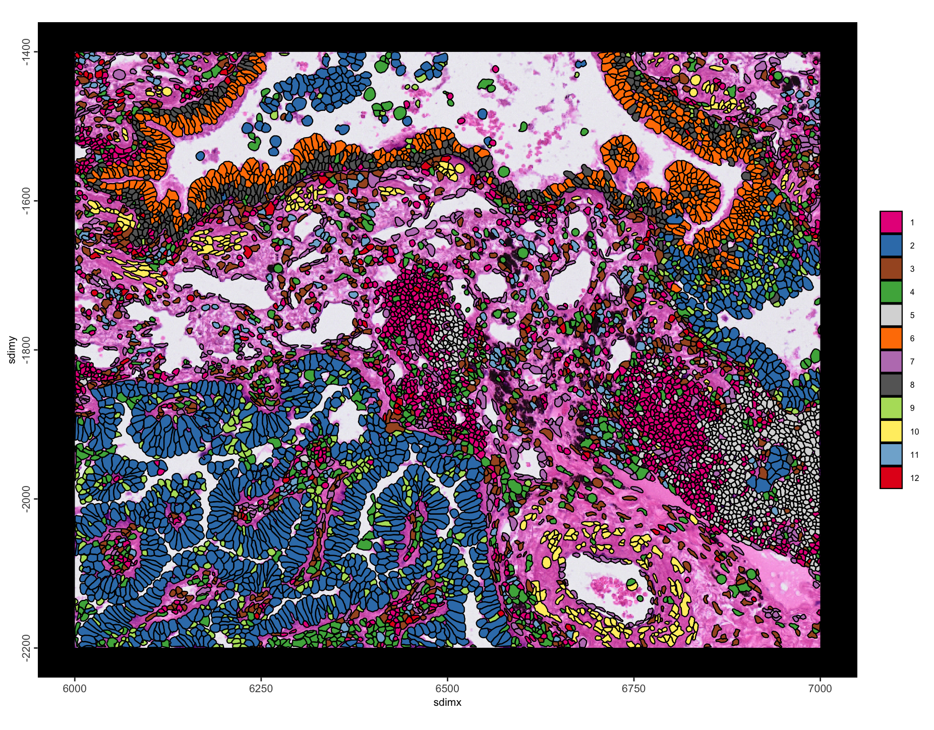
Figure 10.12: Spatial plot with leiden clustering annotations.
10.8 Niche clustering
Building on top of these leiden annotations, we can define spatial niche signatures based on which leiden types are often found together.
10.8.1 Spatial network
First a spatial network must be generated so that spatial relationships between cells can be understood.
g <- createSpatialNetwork(g,
    method = "Delaunay"
)

spatPlot2D(g,
    point_shape = "no_border",
    show_network = TRUE,
    point_size = 0.1,
    point_alpha = 0.5,
    network_color = "grey"
)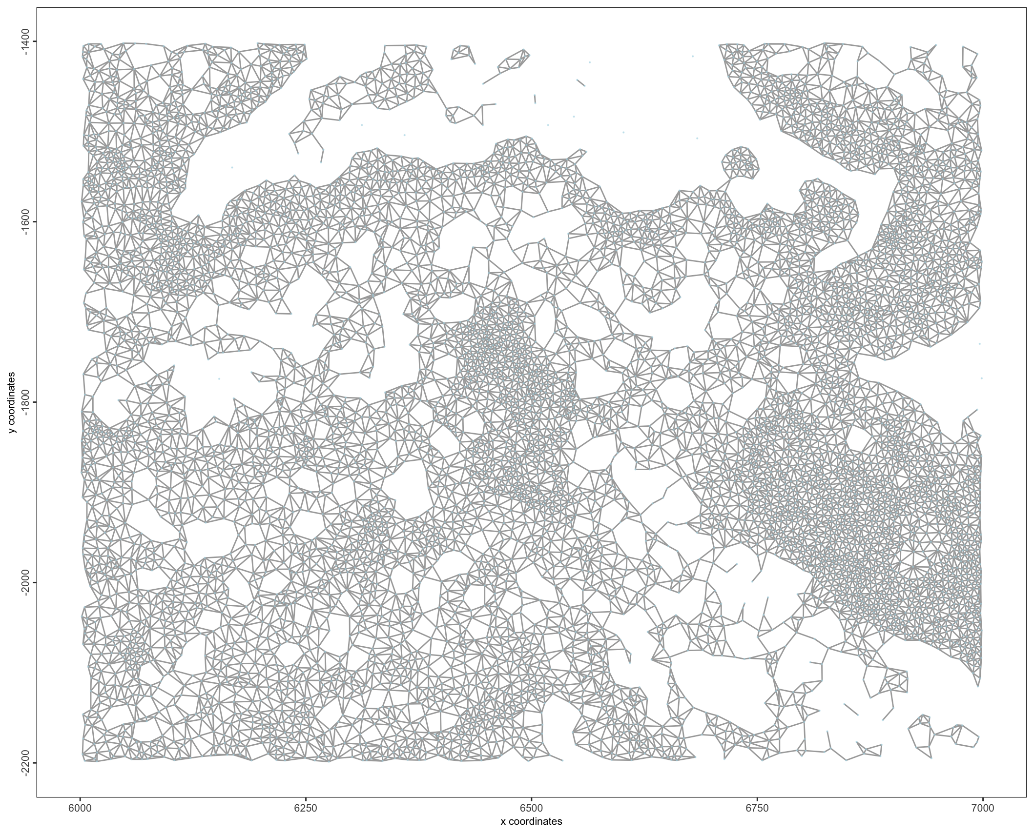
Figure 10.13: Delaunay spatial network`
10.8.2 Niche calculation
Calculate a proportion table for a cell metadata table for all the spatial neighbors of each cell. This means that with each cell established as the center of its local niche, the enrichment of each leiden cluster label is found for that local niche. The results are stored as a new spatial enrichment entry called “leiden_niche”
10.8.3 k-means clustering based on niche signature
# retrieve the niche info
prop_table <- getSpatialEnrichment(g,
    name = "leiden_niche",
    output = "data.table")

# convert to matrix
prop_matrix <- GiottoUtils::dt_to_matrix(prop_table)

# perform kmeans clustering
set.seed(1234) # make kmeans clustering reproducible

prop_kmeans <- kmeans(
    x = prop_matrix,
    centers = 7, # controls how many clusters will be formed
    iter.max = 1000,
    nstart = 100
)

prop_kmeansDT = data.table::data.table(
    cell_ID = names(prop_kmeans$cluster),
    niche = prop_kmeans$cluster
)

# return kmeans clustering on niche to gobject
g <- addCellMetadata(g,
    new_metadata = prop_kmeansDT,
    by_column = TRUE,
    column_cell_ID = "cell_ID"
)

# visualize niches
spatInSituPlotPoints(g,
    show_image = TRUE,
    image_name = "HE",
    polygon_fill = "niche",
    # polygon_fill_code = getColors("Accent", 8),
    polygon_alpha = 1,
    polygon_fill_as_factor = TRUE
)
# visualize niche makeup
cellmeta <- pDataDT(g)
ggplot2::ggplot(
cellmeta, ggplot2::aes(fill = as.character(leiden_clus),
y = 1,
x = as.character(niche))) +
ggplot2::geom_bar(position = "fill", stat = "identity") +
ggplot2::scale_fill_manual(values = c(
"#E7298A", "#FFED6F", "#80B1D3", "#E41A1C", "#377EB8", "#A65628",
"#4DAF4A", "#D9D9D9", "#FF7F00", "#BC80BD", "#666666", "#B3DE69")
)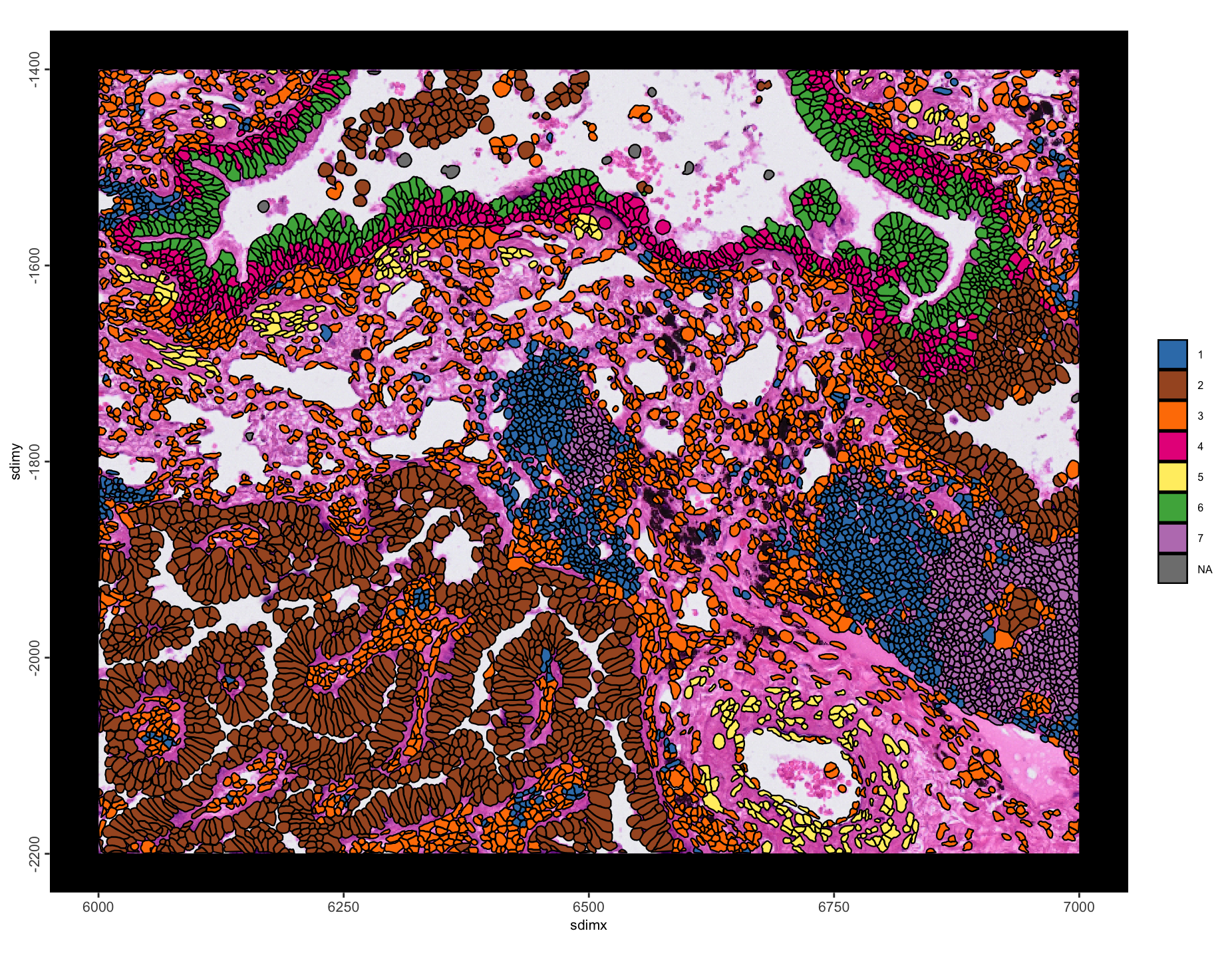
Figure 10.14: Leiden annotation-based spatial niches
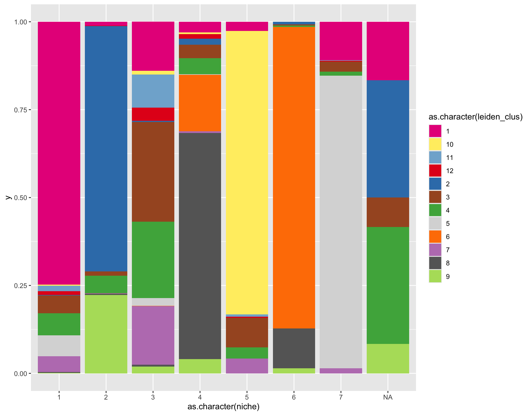
Figure 10.15: Stacked barplot of leiden annotation composition by niche. Coloring is matched to that of the previous spatial plot with leiden clustering annotations
10.9 Cell proximity enrichment
Using a spatial network, determine if there is an enrichment or depletion between annotation types by calculating the observed over the expected frequency of interactions.
# uses a lot of memory
leiden_prox <- cellProximityEnrichment(g,
    cluster_column = "leiden_clus",
    spatial_network_name = "Delaunay_network",
    adjust_method = "fdr",
    number_of_simulations = 2000
)

cellProximityBarplot(g,
    CPscore = leiden_prox,
    min_orig_ints = 5, # minimum original cell-cell interactions
    min_sim_ints = 5 # minimum simulated cell-cell interactions
)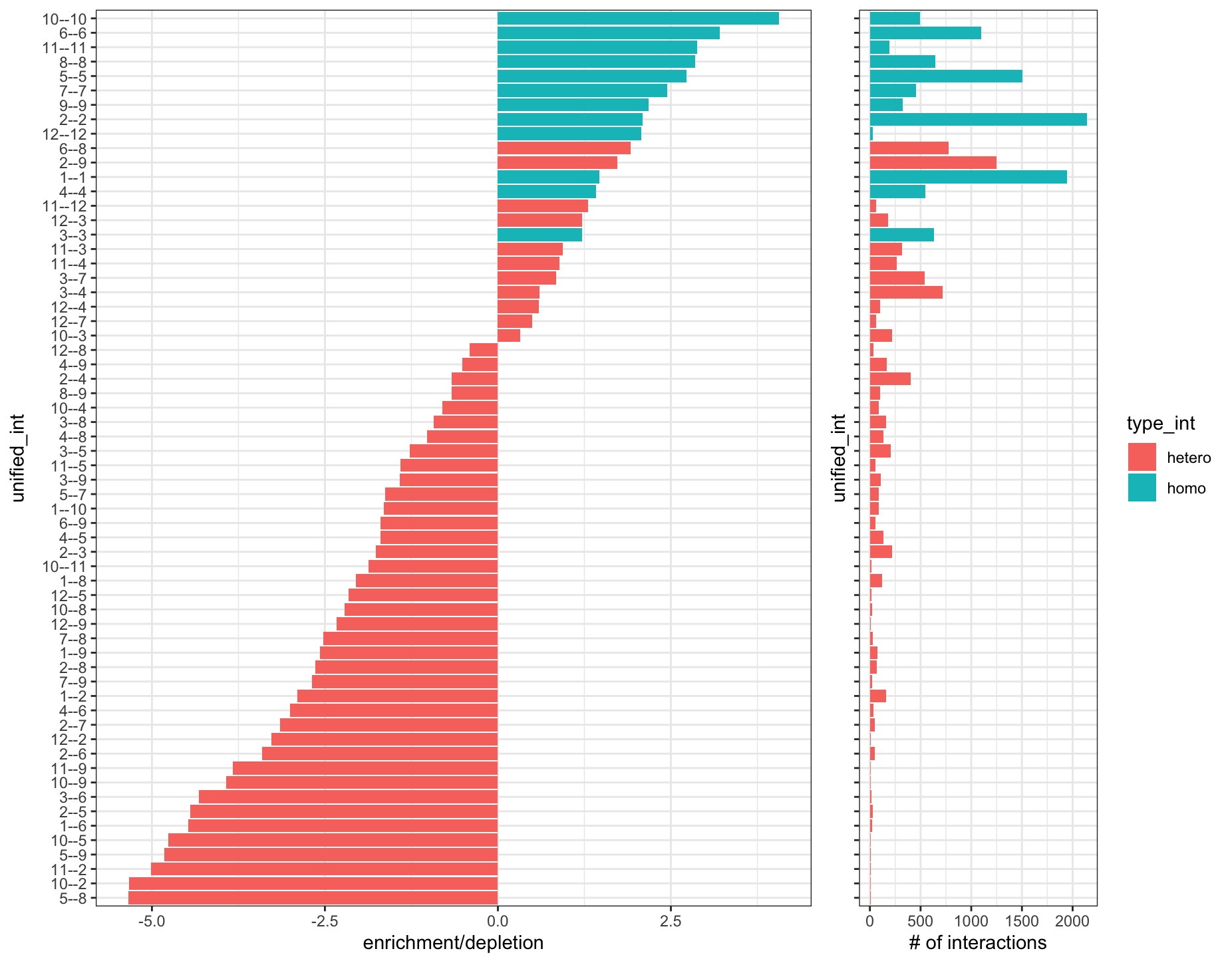
Figure 10.16: Cell-cell interaction enrichments and depletions (left). Number of interactions of each type found (right)
Most enrichments are self-self interactions, which is expected. However, 6–8 and 2–9 stand out as being hetero interactions that are enriched with a large number of interactions. We can take a closer look by plotting these annotation pairs with colors that stand out.
# set up colors
other_cell_color <- rep("grey", 12)
int_6_8 <- int_2_9 <- other_cell_color
int_6_8[c(6, 8)] <- c("orange", "cornflowerblue")
int_2_9[c(2, 9)] <- c("orange", "cornflowerblue")spatInSituPlotPoints(g,
polygon_fill = "leiden_clus",
polygon_fill_as_factor = TRUE,
polygon_fill_code = int_6_8,
polygon_line_size = 0.1,
polygon_alpha = 1,
show_image = TRUE,
image_name = "HE"
)spatInSituPlotPoints(g,
polygon_fill = "leiden_clus",
polygon_fill_as_factor = TRUE,
polygon_fill_code = int_2_9,
polygon_line_size = 0.1,
show_image = TRUE,
polygon_alpha = 1,
image_name = "HE"
)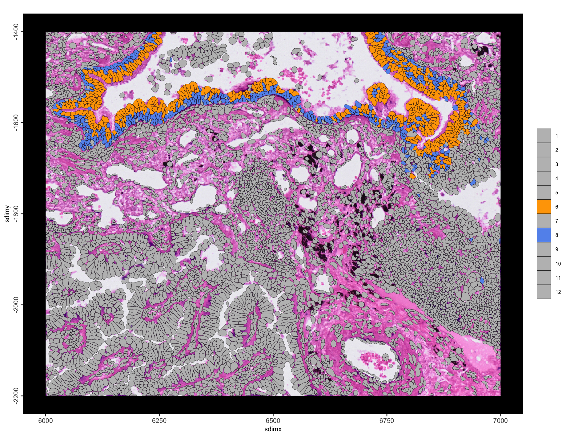
Figure 10.17: Spatial plot of enriched leiden annotation 6 to 8 interactions
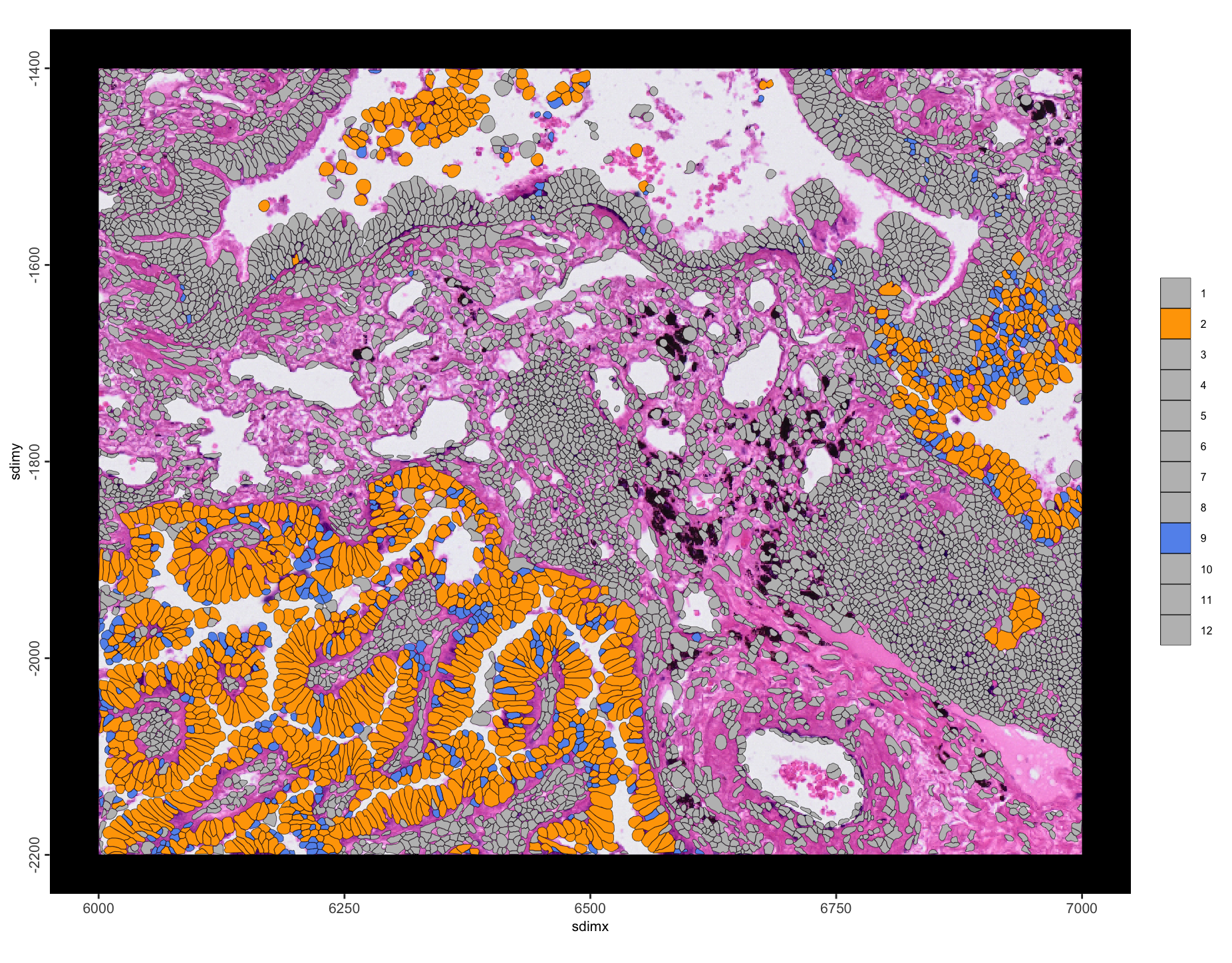
Figure 10.18: Spatial plot of enriched leiden annotation 2 to 9 interactions
10.10 Pseudovisium
Another thing we can do is create a “pseudovisium” dataset by tessellating across this dataset using the same layout and resolution as a Visium capture array.
makePseudoVisium() generates a Visium array of circular polygons across the spatial extent provided.
Here we use ext() with the prefer arg pointing to the polygon and points data and all_data = TRUE, meaning that the combined spatial extent of those two data types will be returned, giving a good measure of where all the data in the object is at the moment.
micron_size = 1 since the Xenium data is already scaled to microns.
pvis <- makePseudoVisium(
    extent = ext(g, prefer = c("polygon", "points"), all_data = TRUE),
     # all_data = TRUE is the default
    micron_size = 1
)

g <- setGiotto(g, pvis)
g <- addSpatialCentroidLocations(g, poly_info = "pseudo_visium")

plot(pvis)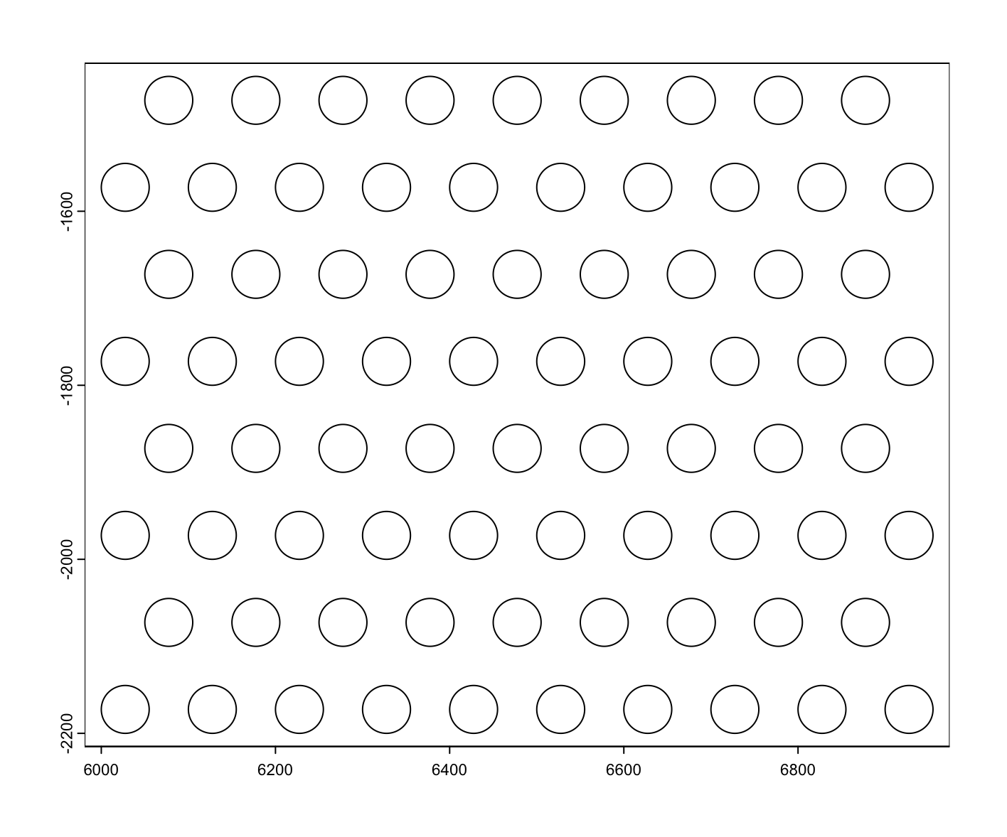
Figure 10.19: Pseudovisium spot geometries generated by makePseudoVisium()
10.10.1 Pseudovisium aggregation and workflow
Make “pseudo_visium” the new default spatial unit then proceed with aggregation and usual aggregate workflow.
activeSpatUnit(g) <- "pseudo_visium"

g <- calculateOverlap(g,
    spatial_info = "pseudo_visium",
    feat_info = "rna"
)

g <- overlapToMatrix(g)

g <- filterGiotto(g,
    expression_threshold = 1,
    feat_det_in_min_cells = 1,
    min_det_feats_per_cell = 100
)

g <- normalizeGiotto(g)

g <- addStatistics(g)

spatInSituPlotPoints(g,
    show_image = TRUE,
    image_name = "HE",
    polygon_feat_type = "pseudo_visium",
    polygon_fill = "total_expr",
    polygon_fill_gradient_style = "sequential"
)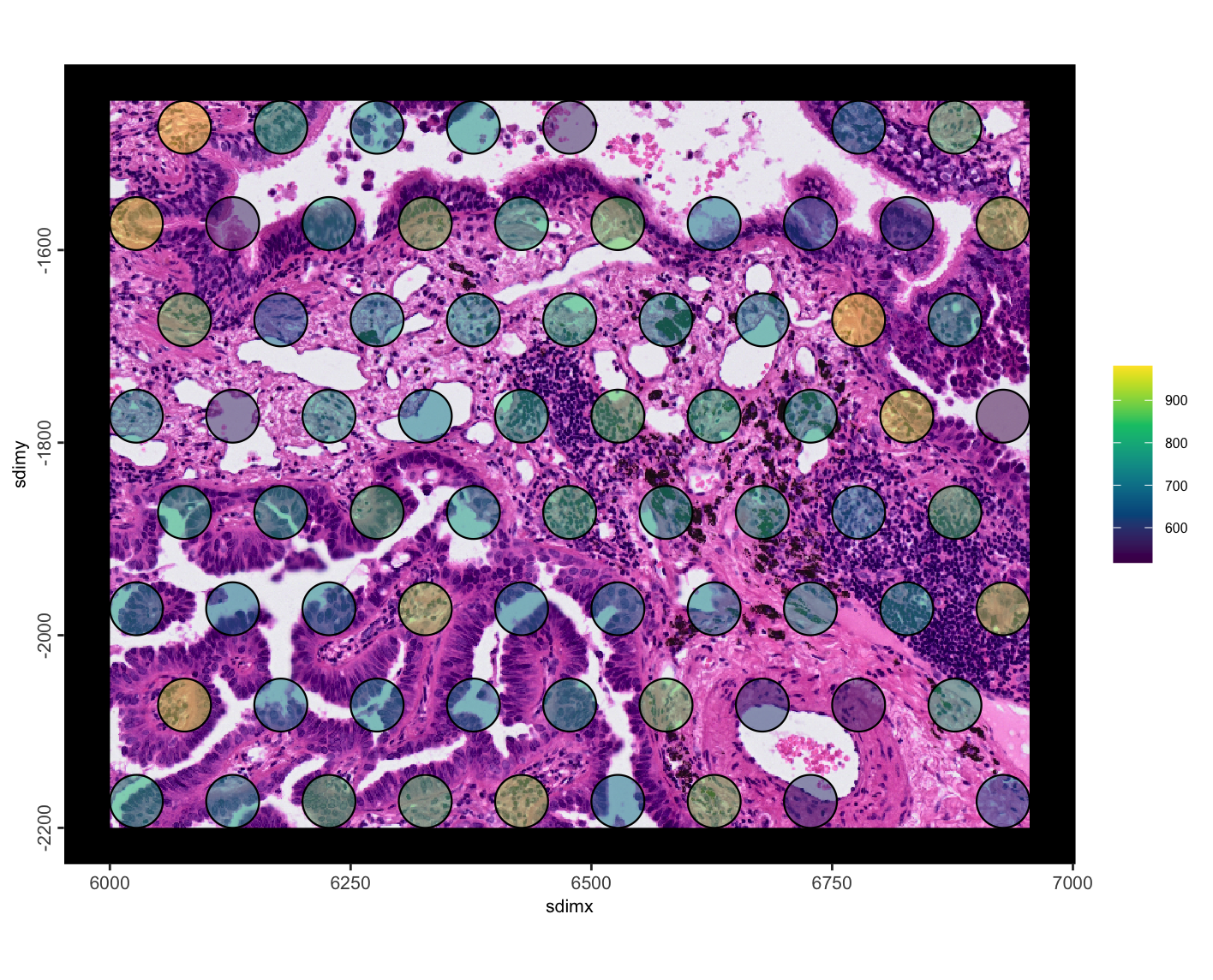
Figure 10.20: Pseudo visium total detections per spot
g <- runPCA(g, feats_to_use = NULL)

g <- runUMAP(g,
    dimensions_to_use = seq(15),
    n_neighbors = 15
)

g <- createNearestNetwork(g,
    dimensions_to_use = seq(15),
    k = 15
)

g <- doLeidenCluster(g, resolution = 1.5)spatInSituPlotPoints(g,
polygon_feat_type = "pseudo_visium",
polygon_fill = "leiden_clus",
polygon_fill_as_factor = TRUE
)spatInSituPlotPoints(g,
polygon_feat_type = "pseudo_visium",
polygon_fill = "leiden_clus",
polygon_fill_as_factor = TRUE,
show_image = TRUE,
image_name = "HE"
)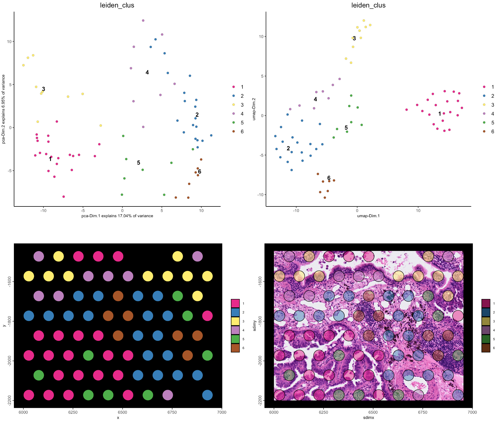
Figure 10.21: Leiden clustering in PCA (top left) and UMAP (top right) spaces, and in spatial plot with no image (bottom left), and with image (bottom right)
