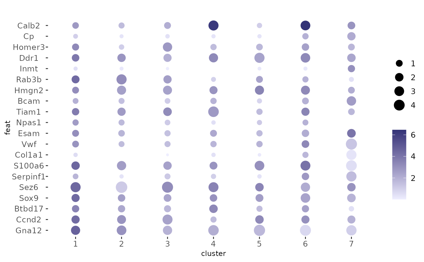
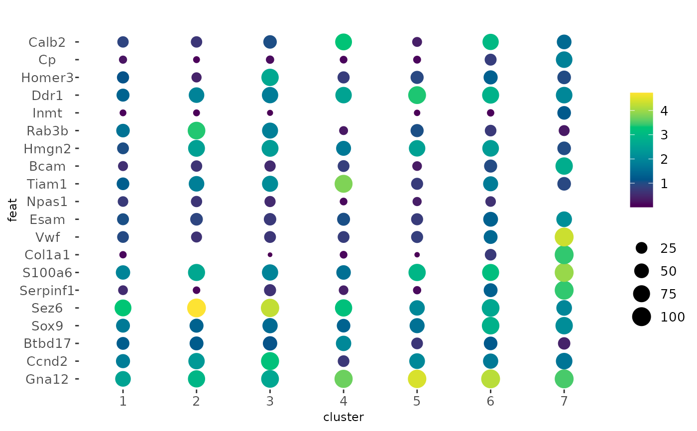
Create a dotplot — dotPlot • GiottoVisuals

Visualize feature expression statistics applied across clusters/groupings of cells. The default behavior is dot size scaled by what percentage of cells within a particular cluster express the feature, and dot color scaled by mean expression of that feature within the cluster.

Usage

dotPlot(
  gobject,
  feats,
  cluster_column,
  cluster_custom_order = NULL,
  dot_size = function(x) mean(x != 0) * 100,
  dot_size_threshold = 0,
  dot_scale = 6,
  dot_color = mean,
  dot_color_gradient = NULL,
  gradient_midpoint = NULL,
  gradient_style = "sequential",
  gradient_limits = NULL,
  group_by = NULL,
  group_by_subset = NULL,
  spat_unit = NULL,
  feat_type = NULL,
  expression_values = c("normalized", "scaled", "custom"),
  title = NULL,
  show_legend = TRUE,
  legend_text = 10,
  legend_symbol_size = 2,
  background_color = "white",
  axis_text = 10,
  axis_title = 9,
  cow_n_col = NULL,
  cow_rel_h = 1,
  cow_rel_w = 1,
  cow_align = "h",
  theme_param = list(),
  show_plot = NULL,
  return_plot = NULL,
  save_plot = NULL,
  save_param = list(),
  default_save_name = "dotPlot"
)

Arguments

gobject: giotto object
feats: character vector or named list. Features to use or named lists of features to use.
cluster_column: character. Clusterings column to use (usually in cell metadata)
cluster_custom_order: character vector. Specific cluster order to use
dot_size, dot_color: summary function e.g. sum, mean, var, or other custom function. The default for dot_size finds the percentage of cells of a particular cluster that do not have an expression level of 0.
dot_size_threshold: numeric. The minimal value at which a dot is no longer drawn.
dot_scale: numeric. Controls size of dots
dot_color_gradient: hex codes or palette name. Color gradient to use.
gradient_midpoint: numeric. midpoint for color gradient
gradient_style: either 'divergent' (midpoint is used in color scaling) or 'sequential' (scaled based on data range)
gradient_limits: numeric vector of length 2. Set minmax value mappings for color gradient
group_by: character. Create multiple plots based on cell annotation column
group_by_subset: character. subset the group_by factor column
spat_unit: spatial unit (e.g. "cell")
feat_type: feature type (e.g. "rna", "dna", "protein")
expression_values: character. Expression values to use.
title: character. title for plot
show_legend: logical. show legend
legend_text: size of legend text
legend_symbol_size: size of legend symbols
background_color: color of plot background
axis_text: size of axis text
axis_title: size of axis title
cow_n_col: cowplot param: how many columns
cow_rel_h: cowplot param: relative heights of rows (e.g. c(1,2))
cow_rel_w: cowplot param: relative widths of columns (e.g. c(1,2))
cow_align: cowplot param: how to align
theme_param: list of additional params passed to ggplot2::theme()
show_plot: logical. show plot
return_plot: logical. return ggplot object
save_plot: logical. save the plot
save_param: list of saving parameters, see showSaveParameters
default_save_name: default save name for saving, don't change, change save_name in save_param

Examples

g <- GiottoData::loadGiottoMini("visium")
#> 1. read Giotto object
#> 2. read Giotto feature information
#> 3. read Giotto spatial information
#> 3.1 read Giotto spatial shape information
#> 3.2 read Giotto spatial centroid information
#> 3.3 read Giotto spatial overlap information
#> 4. read Giotto image information
#> python already initialized in this session
#>  active environment : '/usr/bin/python3'
#>  python version : 3.10
#> checking default envname 'giotto_env'
#> a system default python environment was found
#> Using python path:
#>  "/usr/bin/python3"
library(GiottoClass)
f1 <- head(featIDs(g), 20)
f2 <- tail(featIDs(g), 20)

dotPlot(g, cluster_column = "leiden_clus", feats = f1)


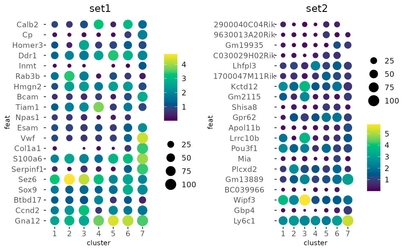
# make two plots from two named sets of features
dotPlot(g,
    cluster_column = "leiden_clus",
    feats = list(set1 = f1, set2 = f2)
)


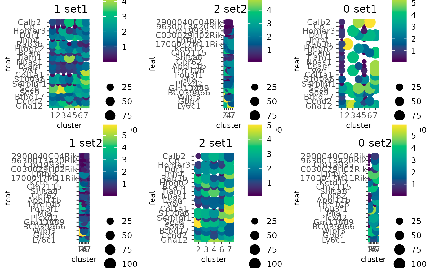
# add new cell metadata col that classifies by total expression into
# - 0 (< 900)
# - 1 (> 900 and < 1200)
# - 2 (> 1200)
total_expr <- g$total_expr
#> Getting values from [cell][rna] cell metadata
g$expr_class <- findInterval(total_expr, c(900, 1200))

# Create a dotplot while splitting the values based on the above total
# expression classifications.
dotPlot(g,
    cluster_column = "leiden_clus",
    feats = list(set1 = f1, set2 = f2),
    group_by = "expr_class"
)


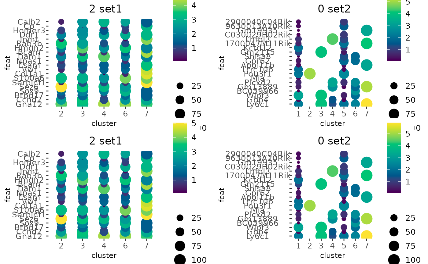
# Same as before, but focusing on classifications 0 and 2
dotPlot(g,
    cluster_column = "leiden_clus",
    feats = list(set1 = f1, set2 = f2),
    group_by = "expr_class",
    group_by_subset = c(0, 2)
)


# example with an alternate function used for `dot_color` and a different
# color gradient
dotPlot(g,
    cluster_column = "leiden_clus",
    feats = f1,
    dot_size = mean,
    dot_color = var,
    dot_color_gradient = c("#EEEEFF", "#333377")
)