Choosing and Creating a Tile Plan

library(tilework)
library(terra)
#> terra 1.9.11

Overview

tilework provides four concrete tile plan classes, each suited to a different way of thinking about how a dataset should be divided:

Class	Tile placement	Coordinate system	Returns
`spatialTilePlan`	Uniform grid	CRS units	`SpatExtent`
`pixelTilePlan`	Uniform grid	Pixel indices	`integer[4]`
`pointTilePlan`	Arbitrary centers	CRS or pixel	`SpatExtent` or `integer[4]`
`freeTilePlan`	Explicit per-tile bounds	Inherent to bounds	`SpatExtent`

The choice between them is usually straightforward:

Working with georeferenced rasters or vectors where coordinates are in CRS units? → spatialTilePlan
Working with images where pixel position is what matters? → pixelTilePlan
Have a list of locations (cell centroids, tissue landmarks, sample sites) you want to extract fixed-size patches around? → pointTilePlan
Need variable-size tiles driven by data density or an external partitioning algorithm? → freeTilePlan (often via quadtreePlan())

`spatialTilePlan`

spatialTilePlan divides a spatial extent into a uniform grid. Tile bounds are returned as SpatExtent objects, which route directly into terra’s spatial windowing operations downstream.

Two things are required: an extent and a tile count request. The actual number of tiles generated will be at least the requested number, arranged as squarely as possible given the extent’s aspect ratio.

tp_spat <- spatialTilePlan(ext = c(0, 1000, 0, 600), n = 12)

tp_spat
#> Object of class spatialTilePlan 
#> extent : 0, 1000, 0, 600 (xmin, xmax, ymin, ymax)
#> dim    : 3 4
#> pad    : 0
dim(tp_spat)   # nrow x ncol of the tile grid
#> [1] 3 4
length(tp_spat)
#> [1] 12

plot(tp_spat)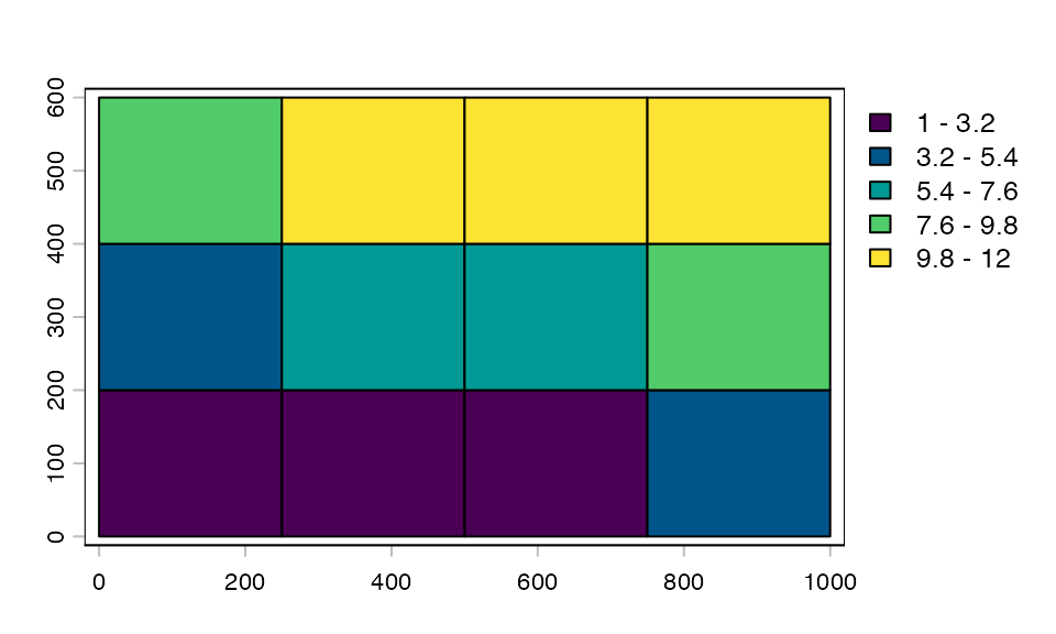

Padding expands each tile’s bounds equally on all four sides at extraction time. The plan’s own extent is not affected.

tp_spat_padded <- tp_spat + 20
plot(tp_spat_padded, alpha = 0.4)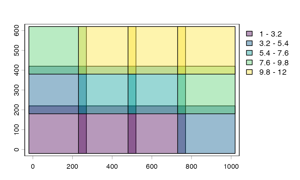

Indexing returns SpatExtent objects:

tp_spat[1]       # first tile
#> [[1]]
#> SpatExtent : 0, 250, 0, 200 (xmin, xmax, ymin, ymax)
tp_spat[2, 3]    # row 2, col 3
#> [[1]]
#> SpatExtent : 500, 750, 200, 400 (xmin, xmax, ymin, ymax)

When to use: Any workflow where tile bounds need to be expressed in the same coordinate system as the data — georeferenced rasters, sf geometries, SpatVector objects.

`pixelTilePlan`

pixelTilePlan divides an image into a uniform grid of pixel-exact tiles. Bounds are returned as integer[4] vectors c(xmin, xmax, ymin, ymax) in pixel index space, routing into array/matrix subsetting operations downstream.

Three things are required: the image’s pixel dimensions (pxdims), and the tile height and width in pixels (nrows, ncols).

tp_px <- pixelTilePlan(pxdims = c(500, 800), nrows = 100, ncols = 100)

tp_px
#> Object of class pixelTilePlan 
#> tiles  : 40
#> pxdim  : 500, 800
#> pxrows : 100
#> pxcol  : 100
#> dim    : 5, 8
#> pad    : 0
dim(tp_px)
#> [1] 5 8
length(tp_px)
#> [1] 40

plot(tp_px)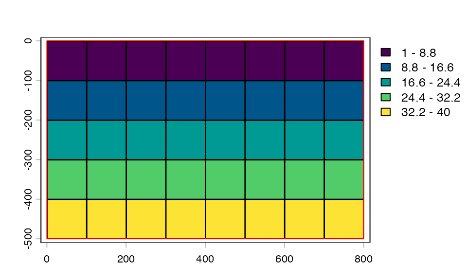

Padding for pixel plans is automatically zeroed against the top-left corner so that padded tiles on the first row/column do not produce negative indices.

tp_px_padded <- tp_px + 5
tp_px_padded[1]   # first tile: note xmin/ymin are still >= 1
#> [[1]]
#> [1]   1 110   1 110
#> attr(,"tile")
#> [1] 1
tp_px[1]          # unpadded for comparison
#> [[1]]
#> [1]   1 100   1 100
#> attr(,"tile")
#> [1] 1

When to use: Image processing workflows where there is no meaningful spatial coordinate system — microscopy images, whole slide images, general computer vision pipelines. Also the right choice when pixel-exact tile boundaries matter (e.g. ML patch extraction where tile size must match model input exactly).

`pointTilePlan`

pointTilePlan places tiles at arbitrary (x, y) centers with a uniform tile size. Instead of dividing a grid, you provide the locations and the plan generates one tile per point.

This is the right choice when the locations to sample are known in advance — cell nuclei, tissue landmarks, sampling sites, feature centroids — rather than when you want to exhaust a spatial extent.

tp_pt <- pointTilePlan("spatial",
    coords = cbind(x = c(100, 250, 400, 550), y = c(80, 200, 150, 300)),
    width  = 80,
    height = 80
)

tp_pt
#> Object of class pointTilePlan 
#> input     : spatial
#> output    : spatial
#> n         : 4
#> tile_dims : 80, 80 (height, width)
#> pad       : 0
length(tp_pt)
#> [1] 4

plot(tp_pt)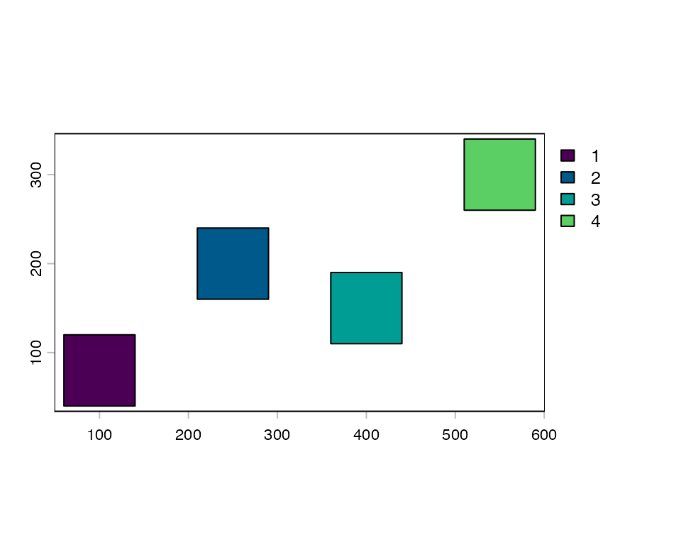

Coordinate modes: `input` and `output`

pointTilePlan has two independent coordinate mode settings:

$input — the space in which $coords, $width, and $height are expressed. Either "spatial" (CRS units) or "pixel" (pixel indices).
$output — the type of bounds returned by getTile(). Either "spatial" (returns SpatExtent) or "pixel" (returns integer[4]).

By default output matches input. Setting them to different values enables cross-mode conversion.

The four combinations:

`input`	`output`	Meaning
`"spatial"`	`"spatial"`	Spatial coords in, spatial bounds out
`"pixel"`	`"pixel"`	Pixel coords in, pixel bounds out
`"spatial"`	`"pixel"`	Define location in CRS, extract pixel bounds
`"pixel"`	`"spatial"`	Define location in pixel space, extract spatial bounds

Same-mode: spatial → spatial

The most common case. Coordinates, tile dims, and padding are all in CRS units. No raster metadata needed.

tp_s2s <- pointTilePlan(input = "spatial", output = "spatial",
    coords = cbind(x = c(200, 500), y = c(150, 400)),
    width  = 100,
    height = 100
)

tp_s2s[1]  # SpatExtent
#> [[1]]
#> SpatExtent : 150, 250, 100, 200 (xmin, xmax, ymin, ymax)

Same-mode: pixel → pixel

Coordinates and tile dims are in pixel indices. Useful when sampling locations come from image analysis (e.g. detected cell positions in pixel space).

tp_p2p <- pointTilePlan(input = "pixel", output = "pixel",
    coords = cbind(x = c(120L, 340L, 560L), y = c(80L, 200L, 310L)),
    width  = 51L,   # odd dims give unambiguous center pixel
    height = 51L
)

tp_p2p[2]  # integer[4]: col_min, col_max, row_min, row_max
#> [[1]]
#> [1] 315 365 175 225
#> attr(,"tile")
#> [1] 2
#> attr(,"x")
#> [1] 340
#> attr(,"y")
#> [1] 200

Note: tile dims should be odd in pixel mode. With even dimensions, center ± width/2 is non-integer and bounds are truncated, biasing left/up.

Cross-mode: spatial → pixel and pixel → spatial

Cross-mode conversion requires knowing how CRS coordinates map to pixel indices, which means the raster’s resolution and extent must be known.

When getTile() is called with a SpatRaster, this information is injected automatically from the raster — you do not need to set $rast_dims or $extent manually. They are only needed for standalone [i] calls without a raster (e.g. plotting, validation).

f <- system.file("ex/elev.tif", package = "terra")
r <- rast(f)

# spatial input, pixel output
tp_s2p <- pointTilePlan(input = "spatial", output = "pixel",
    coords = cbind(x = c(5.8, 6.0, 6.2), y = c(49.9, 50.0, 50.1)),
    width  = 0.1,
    height = 0.1
)

# Standalone [i] requires rast_dims and extent:
tp_s2p$rast_dims <- dim(r)[1:2]
tp_s2p$extent    <- as.vector(ext(r))

tp_s2p[1]  # pixel bounds, derived from spatial coords + raster metadata
#> [[1]]
#> [1]  9  8 36 35
#> attr(,"tile")
#> [1] 1
#> attr(,"x")
#> [1] 5.8
#> attr(,"y")
#> [1] 49.9

# At getTile() time, rast_dims and extent are injected from the raster
# automatically — no manual setup needed for the extraction step:
tiles <- getTile(r, tp_s2p, i = 1:3)
dim(tiles[[1]])
#> [1] 2 2 1

`freeTilePlan` and `quadtreePlan`

freeTilePlan stores explicit per-tile bounds as an n × 4 matrix (xmin, xmax, ymin, ymax). Unlike the grid-based plans, tile sizes can vary freely — bounds are the canonical representation, not a formula.

The simplest use is to supply bounds directly:

tp_free <- freeTilePlan()
tp_free$bounds <- rbind(
    c(0,  50,  0,  50),
    c(50, 100, 0,  50),
    c(0,  50,  50, 100),
    c(50, 100, 50, 100)
)

tp_free
#> Object of class freeTilePlan 
#> n      : 4
#> xrange : [0, 100]
#> yrange : [0, 100]
#> pad    : 0
length(tp_free)
#> [1] 4
tp_free[2]   # SpatExtent
#> [[1]]
#> SpatExtent : 50, 100, 0, 50 (xmin, xmax, ymin, ymax)

plot(tp_free)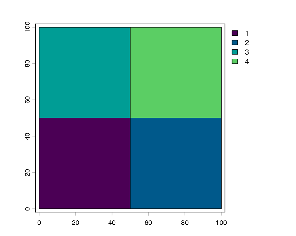

Adaptive decomposition with `quadtreePlan()`

The more common workflow is to let quadtreePlan() build the freeTilePlan automatically. It starts from a coarse tilePlan, applies FUN to each tile, and recursively splits tiles whose value exceeds threshold. Splitting continues until all tiles are below the threshold, smaller than min_tile_size, or max_depth is reached. After splitting, neighboring leaf tiles whose combined FUN value stays ≤ threshold are merged back into a single rectangle, reducing tile count in sparse regions.

FUN must return a single numeric scalar per tile — typically a count, density, or variance. The last measured value for each leaf is stored in the n_records metadata column.

# Synthetic two-cluster point cloud
set.seed(42)
pts <- terra::vect(
    cbind(x = rnorm(1000, 0, 50), y = rnorm(1000, 0, 50))
)
pts <- rbind(pts, terra::vect(
    cbind(x = rnorm(1000, 300, 50), y = rnorm(1000, 300, 50))
))

# tileApply requires on-disk data
f_pts <- tempfile(fileext = ".shp")
terra::writeVector(pts, f_pts)
pts_proxy <- terra::vect(f_pts, proxy = TRUE)

# Coarse 2×2 starting grid
tp_start <- spatialTilePlan(ext = ext(pts), n = 4L)
tp_start
#> Object of class spatialTilePlan 
#> extent : -168.586954127526, 473.545480173295, -146.423858928878, 458.725989214004 (xmin, xmax, ymin, ymax)
#> dim    : 2 2
#> pad    : 0

fp <- quadtreePlan(
    x             = pts_proxy,
    tiles         = tp_start,
    FUN           = function(x) length(x),   # point count per tile
    threshold     = 300L,
    min_tile_size = 10
)
#> Warning: Your code is running sequentially. For better performance, consider using a
#>  parallel plan like:
#>   future::plan(future::multisession)
#>   To silence this warning, set options("tilework.warn_sequential" = FALSE)
#> Warning: Your code is running sequentially. For better performance, consider using a
#>  parallel plan like:
#>   future::plan(future::multisession)
#>   To silence this warning, set options("tilework.warn_sequential" = FALSE)
#> Warning: Your code is running sequentially. For better performance, consider using a
#>  parallel plan like:
#>   future::plan(future::multisession)
#>   To silence this warning, set options("tilework.warn_sequential" = FALSE)
fp
#> Object of class freeTilePlan 
#> n      : 12
#> xrange : [-168.587, 473.545]
#> yrange : [-146.424, 458.726]
#> pad    : 0
length(fp)
#> [1] 12

plot(fp)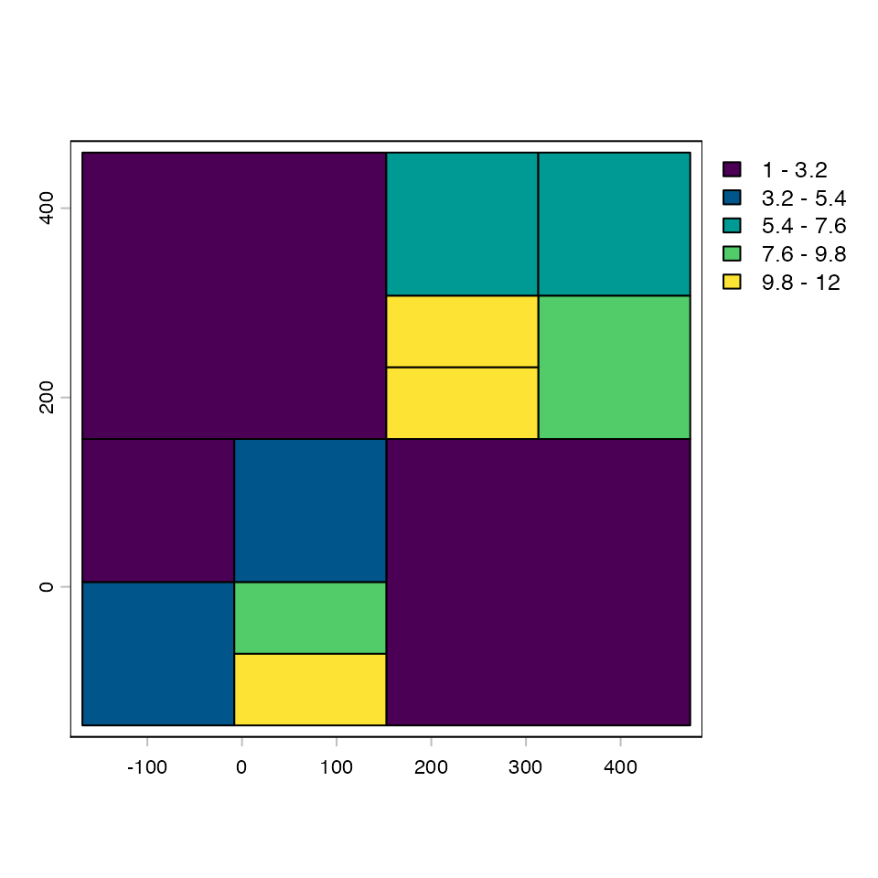

High-density regions are subdivided into many small tiles; sparse regions remain as large tiles (or are merged back if neighbors are also sparse). n_records records the point count for each leaf:

summary(fp$n_records)
#>    Min. 1st Qu.  Median    Mean 3rd Qu.    Max. 
#>     4.0    48.5   219.0   166.7   244.5   284.0

plot(fp, values = "n_records")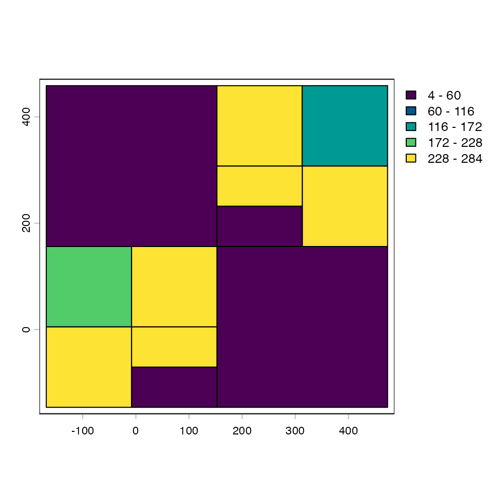

The resulting freeTilePlan is a standard tilePlan and works with tileApply(), tileIterator, and tileGroup like any other.

When to use:

Vector/point data where density varies strongly across space.
Any workflow where a uniform grid would waste computation in empty regions or exceed memory limits in dense regions.
As the output of an external space-partitioning step (pass bounds directly via $bounds<-).

Limitations: @tile_dims is not populated, so operations that require uniform tile dimensions (e.g. extend = TRUE in getTile()) are not supported.

Choosing tile size and padding

Regardless of plan type, two practical considerations apply:

Tile size controls the memory footprint per tile and, for ML workflows, should be chosen with the model’s expected input dimensions in mind. Larger tiles mean fewer total tiles but more memory per tile. If the natural tile size does not match the model input exactly, terra::aggregate() or terra::resample() can resize the extracted tile inside FUN rather than constraining the tile plan itself.

Padding handles edge effects for operations that need spatial context (convolutions, focal statistics, buffer-based extractions). The pad value should be at least as large as the half-width of the operation’s kernel or buffer radius. For pixel plans, padding is zero-clamped at image edges; for spatial plans it extends beyond the plan extent, so shrink the plan extent inward by the pad amount if you want tiles to stay within the data boundary.

tp_demo <- spatialTilePlan(ext = c(0, 100, 0, 100), n = 9)

# shrink extent inward by pad so padded tiles stay within data
pad <- 3
ext(tp_demo) <- ext(tp_demo) - pad
tp_demo <- tp_demo + pad

plot(tp_demo, alpha = 0.4)
plot(ext(c(0, 100, 0, 100)), add = TRUE, border = "red")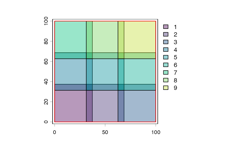

Summary

Plan	Tile placement	Coordinate system	Returns	Primary use case
spatialTilePlan	Uniform grid	CRS units	SpatExtent	Georeferenced rasters and vectors
pixelTilePlan	Uniform grid	Pixel indices	integer[4]	Images, ML patch extraction
pointTilePlan	Arbitrary centers	CRS or pixel (configurable)	SpatExtent or integer[4]	Sampling at known locations
freeTilePlan	Explicit per-tile bounds	Inherent to bounds	SpatExtent	Adaptive/variable-size tiling; quadtree decomposition

Overview

spatialTilePlan

pixelTilePlan

pointTilePlan

Coordinate modes: input and output