Interactive visualization with vitessceR
Source:vignettes/interactive_giotto_vitessceR.Rmd
interactive_giotto_vitessceR.RmdWe have created a function that facilitates the interaction with the vitessceR package for interactive visualization of processed datasets.
1 Set up the Giotto enviroment
# Ensure Giotto Suite is installed.
if(!"Giotto" %in% installed.packages()) {
  pak::pkg_install("drieslab/Giotto")
}

# Ensure GiottoData, a small, helper module for tutorials, is installed.
if(!"GiottoData" %in% installed.packages()) {
  pak::pkg_install("drieslab/GiottoData")
}

library(Giotto)

# Ensure the Python environment for Giotto has been installed.
genv_exists <- checkGiottoEnvironment()
if(!genv_exists){
  # The following command need only be run once to install the Giotto environment.
  installGiottoEnvironment()
}
2 Install the vitessceR package
pak::pkg_install("vitessce/vitessceR")3 Load a mini Giotto object
For this tutorial, we will work with two mini objects: the mini visium and mini vizgen datasets.
visium_object <- GiottoData::loadGiottoMini("visium")

vizgen_object <- GiottoData::loadGiottoMini("vizgen")
4 Export the Giotto object to a local Anndata-Zarr folder
By default, the function giottoToAnndataZarr() will look for the “cell” spatial unit and “rna” feature type, but you can specify the spat_unit and feat_type arguments, as well as the expression values to use.
In addition, you need to specify the path or name for creating a new folder that will store the Anndata-Zarr information.
5 Create the vitessceR object
To create the vitessceR object, you need to provide the paths for the metadata information that you want to load from your Anndata-Zarr folder. We suggest to explore the subfolders obs (for cell metadata), var (for feature metadata), and obsm (for spatial and dimension reduction data).
library(vitessceR)

w <- AnnDataWrapper$new(
  adata_path = "visium_anndata_zarr",
  obs_feature_matrix_path = "X",
  obs_set_paths = c("obs/leiden_clus", "obs/custom_leiden"),
  obs_set_names = c("Leiden clusters", "Custom Leiden clusters"),
  obs_locations_path = "obsm/spatial",
  obs_embedding_paths = c("obsm/spatial", "obsm/pca", "obsm/tsne", "obsm/umap"),
  obs_embedding_names = c("Spatial", "PCA",  "t-SNE", "UMAP"),
  feature_labels_path = "var/feat_ID",
  obs_labels_paths = "obs/cell_ID",
  obs_labels_names = "cell_ID",
)

w <- AnnDataWrapper$new(
  adata_path = "vizgen_anndata_zarr",
  obs_feature_matrix_path = "X",
  obs_set_paths = c("obs/leiden_clus", "obs/louvain_clus"),
  obs_set_names = c("Leiden clusters", "Louvain clusters"),
  obs_locations_path = "obsm/spatial",
  obs_embedding_paths = c("obsm/spatial", "obsm/pca", "obsm/tsne", "obsm/umap"),
  obs_embedding_names = c("Spatial", "PCA", "t-SNE", "UMAP"),
  feature_labels_path = "var/feat_ID",
  obs_labels_paths = "obs/cell_ID",
  obs_labels_names = "cell_ID"
)
6 Create the vitessceR schema
Here we will create the base of the schema using the previous object, then we will add the components to generate interactive plots.
vc <- VitessceConfig$new(schema_version = "1.0.16", name = "My config")
dataset <- vc$add_dataset("My dataset")$add_object(w)
cluster_sets <- vc$add_view(dataset, Component$OBS_SETS)
features <- vc$add_view(dataset, Component$FEATURE_LIST)
scatterplot_spatial <- vc$add_view(dataset, Component$SCATTERPLOT, mapping = "Spatial")
scatterplot_pca <- vc$add_view(dataset, Component$SCATTERPLOT, mapping = "PCA")
scatterplot_umap <- vc$add_view(dataset, Component$SCATTERPLOT, mapping = "UMAP")
scatterplot_tsne <- vc$add_view(dataset, Component$SCATTERPLOT, mapping = "t-SNE")
desc <- vc$add_view(dataset, Component$DESCRIPTION)
desc <- desc$set_props(description = "Visualization of a Giotto object.")
7 Create the layout
You can create multi-column layout and add more compartments using the horizontal (hconcat) or vertical (vconcat) sections.
vc$layout(
  hconcat(
    vconcat(
      hconcat(desc, cluster_sets),
      features,
      scatterplot_spatial
      ),
    vconcat(
      scatterplot_pca,
      scatterplot_umap,
      scatterplot_tsne)
  )
)
8 Render the Vitessce widget
vc$widget(theme = "light")The default view will color the points using the first column defined in the obs_set_paths section, in this case is the Leiden clusters column.
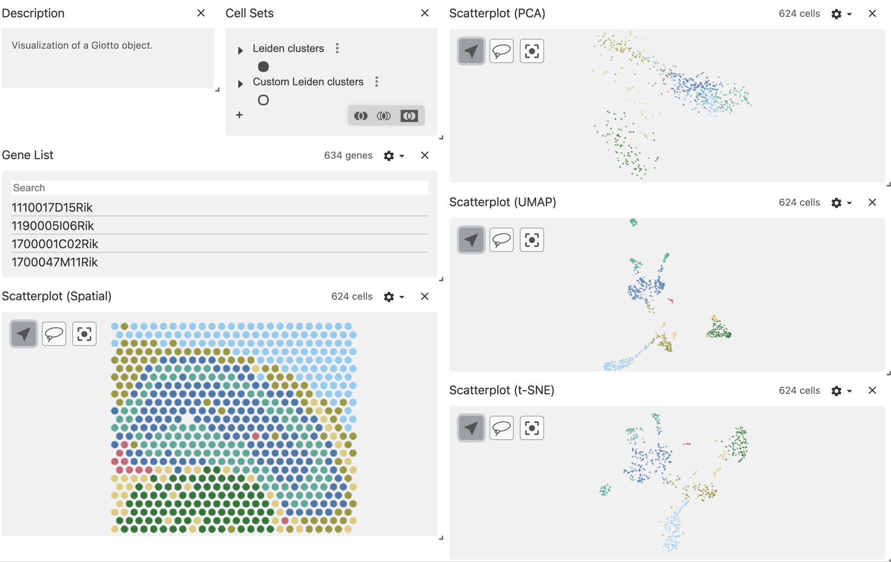
mini visium object
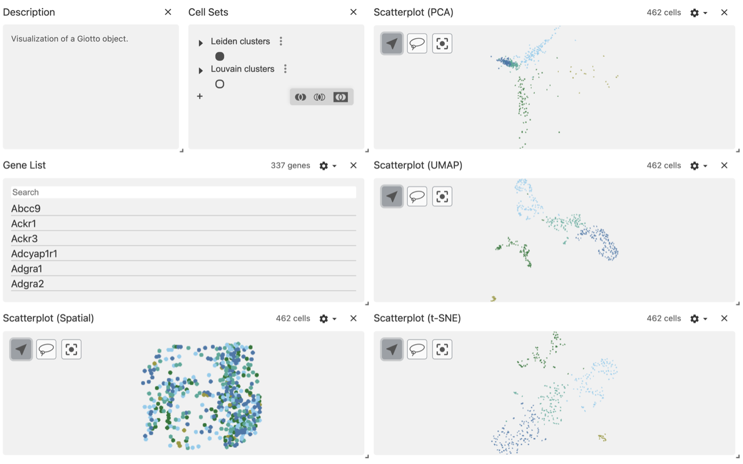
mini vizgen object
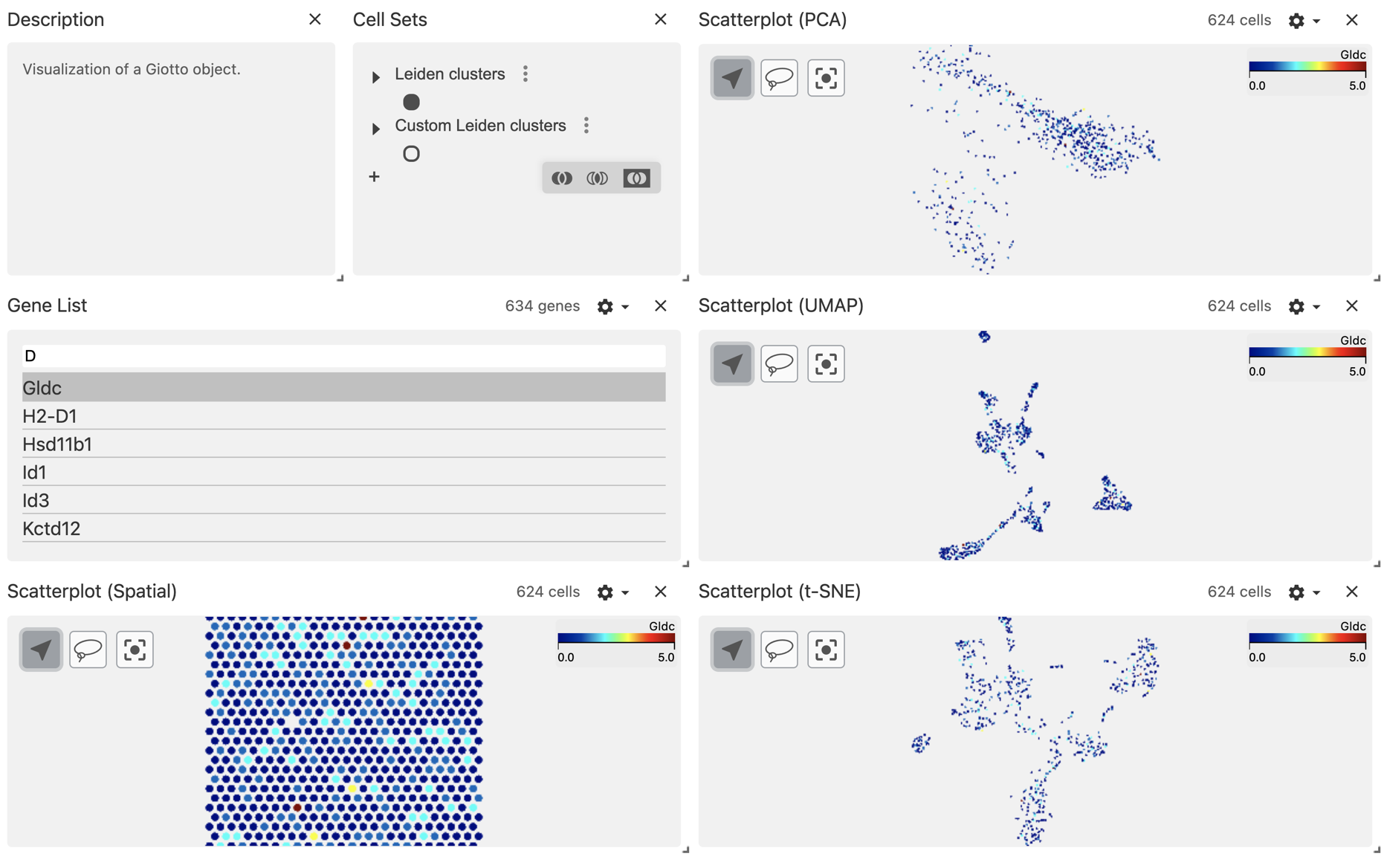
Using the configuration wheel, you can choose to color the points using the gene expression values instead.
9 Session info
R version 4.4.1 (2024-06-14)
Platform: x86_64-apple-darwin20
Running under: macOS Sonoma 14.6.1

Matrix products: default
BLAS:   /System/Library/Frameworks/Accelerate.framework/Versions/A/Frameworks/vecLib.framework/Versions/A/libBLAS.dylib
LAPACK: /Library/Frameworks/R.framework/Versions/4.4-x86_64/Resources/lib/libRlapack.dylib;  LAPACK version 3.12.0

locale:
[1] en_US.UTF-8/en_US.UTF-8/en_US.UTF-8/C/en_US.UTF-8/en_US.UTF-8

time zone: America/New_York
tzcode source: internal

attached base packages:
[1] stats     graphics  grDevices utils     datasets  methods   base

other attached packages:
[1] vitessceR_0.99.0  Giotto_4.1.3      GiottoClass_0.4.0

loaded via a namespace (and not attached):
  [1] RcppAnnoy_0.0.22            splines_4.4.1               later_1.3.2
  [4] filelock_1.0.3              tibble_3.2.1                R.oo_1.26.0
  [7] polyclip_1.10-7             basilisk.utils_1.16.0       fastDummies_1.7.4
 [10] lifecycle_1.0.4             rprojroot_2.0.4             globals_0.16.3
 [13] lattice_0.22-6              MASS_7.3-60.2               backports_1.5.0
 [16] magrittr_2.0.3              plotly_4.10.4               yaml_2.3.10
 [19] httpuv_1.6.15               Seurat_5.1.0                sctransform_0.4.1
 [22] spam_2.10-0                 sp_2.1-4                    spatstat.sparse_3.1-0
 [25] reticulate_1.39.0           cowplot_1.1.3               pbapply_1.7-2
 [28] RColorBrewer_1.1-3          abind_1.4-5                 zlibbioc_1.50.0
 [31] Rtsne_0.17                  GenomicRanges_1.56.1        purrr_1.0.2
 [34] R.utils_2.12.3              BiocGenerics_0.50.0         rappdirs_0.3.3
 [37] GenomeInfoDbData_1.2.12     IRanges_2.38.1              S4Vectors_0.42.1
 [40] ggrepel_0.9.6               irlba_2.3.5.1               listenv_0.9.1
 [43] spatstat.utils_3.1-0        terra_1.7-78                goftest_1.2-3
 [46] RSpectra_0.16-2             spatstat.random_3.3-1       fitdistrplus_1.2-1
 [49] parallelly_1.38.0           webutils_1.2.1              leiden_0.4.3.1
 [52] colorRamp2_0.1.0            codetools_0.2-20            DelayedArray_0.30.1
 [55] tidyselect_1.2.1            farver_2.1.2                UCSC.utils_1.0.0
 [58] matrixStats_1.4.1           stats4_4.4.1                spatstat.explore_3.3-2
 [61] GiottoData_0.2.13           jsonlite_1.8.8              progressr_0.14.0
 [64] ggridges_0.5.6              survival_3.6-4              dbscan_1.2-0
 [67] tools_4.4.1                 ica_1.0-3                   Rcpp_1.0.13
 [70] glue_1.7.0                  gridExtra_2.3               SparseArray_1.4.8
 [73] here_1.0.1                  MatrixGenerics_1.16.0       GenomeInfoDb_1.40.1
 [76] dplyr_1.1.4                 withr_3.0.1                 fastmap_1.2.0
 [79] basilisk_1.16.0             fansi_1.0.6                 digest_0.6.37
 [82] R6_2.5.1                    mime_0.12                   colorspace_2.1-1
 [85] scattermore_1.2             gtools_3.9.5                tensor_1.5
 [88] spatstat.data_3.1-2         R.methodsS3_1.8.2           utf8_1.2.4
 [91] tidyr_1.3.1                 generics_0.1.3              data.table_1.16.0
 [94] httr_1.4.7                  htmlwidgets_1.6.4           S4Arrays_1.4.1
 [97] uwot_0.2.2                  pkgconfig_2.0.3             gtable_0.3.5
[100] lmtest_0.9-40               GiottoVisuals_0.2.5         SingleCellExperiment_1.26.0
[103] XVector_0.44.0              htmltools_0.5.8.1           dotCall64_1.1-1
[106] swagger_5.17.14.1           SeuratObject_5.0.2          scales_1.3.0
[109] Biobase_2.64.0              SeuratData_0.2.2.9001       GiottoUtils_0.1.12
[112] png_0.1-8                   SpatialExperiment_1.14.0    spatstat.univar_3.0-1
[115] plumber_1.2.2               rstudioapi_0.16.0           reshape2_1.4.4
[118] rjson_0.2.22                checkmate_2.3.2             nlme_3.1-164
[121] zoo_1.8-12                  stringr_1.5.1               KernSmooth_2.23-24
[124] parallel_4.4.1              miniUI_0.1.1.1              pillar_1.9.0
[127] grid_4.4.1                  vctrs_0.6.5                 RANN_2.6.2
[130] promises_1.3.0              xtable_1.8-4                cluster_2.1.6
[133] magick_2.8.4                cli_3.6.3                   compiler_4.4.1
[136] rlang_1.1.4                 crayon_1.5.3                vitessceAnalysisR_0.99.0
[139] future.apply_1.11.2         labeling_0.4.3              plyr_1.8.9
[142] stringi_1.8.4               viridisLite_0.4.2           deldir_2.0-4
[145] munsell_0.5.1               lazyeval_0.2.2              spatstat.geom_3.3-2
[148] Matrix_1.7-0                dir.expiry_1.12.0           RcppHNSW_0.6.0
[151] patchwork_1.2.0             future_1.34.0               ggplot2_3.5.1
[154] shiny_1.9.1                 SummarizedExperiment_1.34.0 ROCR_1.0-11
[157] igraph_2.0.3