1 Dataset explanation
10x Genomics obtained fresh frozen mouse kidney tissue (Strain C57BL/6)from BioIVT Asterand. The tissue was embedded and cryosectioned as described in Visium Spatial Protocols - Tissue Preparation Guide (Demonstrated Protocol CG000240). Tissue sections of 10 µm thickness were placed on Visium Gene Expression Slides.
The Visium kidney data to run this tutorial can be found here
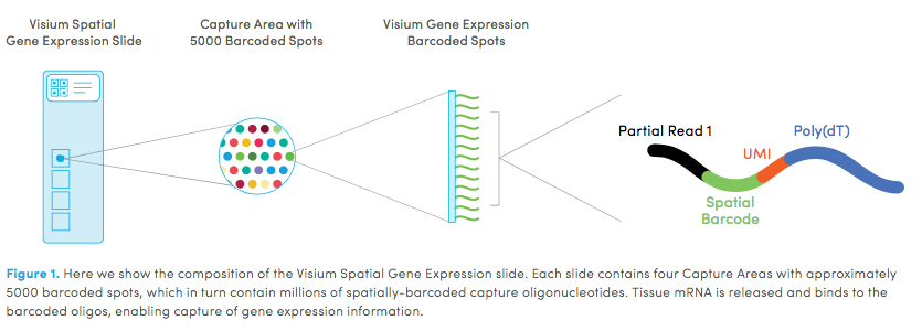
Visium technology:
2 Set up Giotto Environment
# Ensure Giotto Suite is installed.
if (!"Giotto" %in% installed.packages()) {
    pak::pkg_install("drieslab/Giotto")
}

# Ensure the Python environment for Giotto has been installed.
genv_exists <- Giotto::checkGiottoEnvironment()

if (!genv_exists) {
    # The following command need only be run once to install the Giotto environment.
    Giotto::installGiottoEnvironment()
}
3 Giotto global instructions and preparations
library(Giotto)

# 1. set working directory
results_folder <- "/path/to/results/"

# Optional: Specify a path to a Python executable within a conda or miniconda
# environment. If set to NULL (default), the Python executable within the previously
# installed Giotto environment will be used.
python_path <- NULL # alternatively, "/local/python/path/python" if desired.
## create instructions
instructions <- createGiottoInstructions(save_dir = results_folder,
                                         save_plot = TRUE,
                                         show_plot = FALSE,
                                         return_plot = FALSE,
                                         python_path = python_path)

## provide path to visium folder
data_path <- "/path/to/data/"
4 Create Giotto object & process data
## directly from visium folder
visium_kidney <- createGiottoVisiumObject(
    visium_dir = data_path,
    expr_data = "raw",
    png_name = "tissue_lowres_image.png",
    gene_column_index = 2,
    instructions = instructions
)

## check metadata
pDataDT(visium_kidney)

# check available image names
showGiottoImageNames(visium_kidney) # "image" is the default name

## show aligned image
spatPlot(gobject = visium_kidney,
         cell_color = "in_tissue",
         show_image = TRUE,
         point_alpha = 0.7)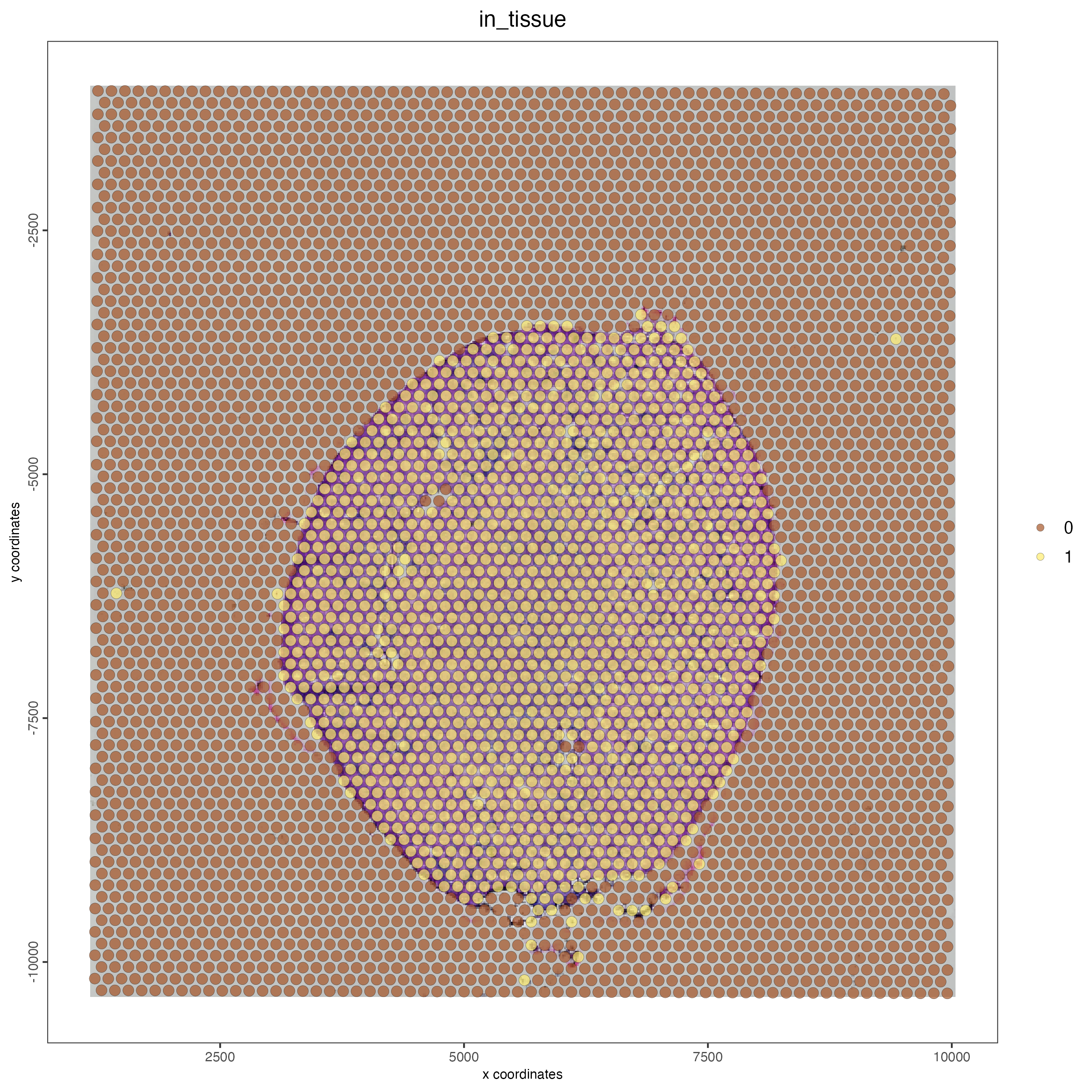
## subset on spots that were covered by tissue
metadata <- pDataDT(visium_kidney)
in_tissue_barcodes <- metadata[in_tissue == 1]$cell_ID

visium_kidney <- subsetGiotto(visium_kidney,
                              cell_ids = in_tissue_barcodes)

## filter
visium_kidney <- filterGiotto(
    gobject = visium_kidney,
    expression_threshold = 1,
    feat_det_in_min_cells = 50,
    min_det_feats_per_cell = 1000,
    expression_values = "raw",
    verbose = TRUE
)

## normalize
visium_kidney <- normalizeGiotto(gobject = visium_kidney,
                                 scalefactor = 6000,
                                 verbose = TRUE)

## add gene & cell statistics
visium_kidney <- addStatistics(gobject = visium_kidney)

## visualize
spatPlot2D(gobject = visium_kidney,
           show_image = TRUE,
           point_alpha = 0.7)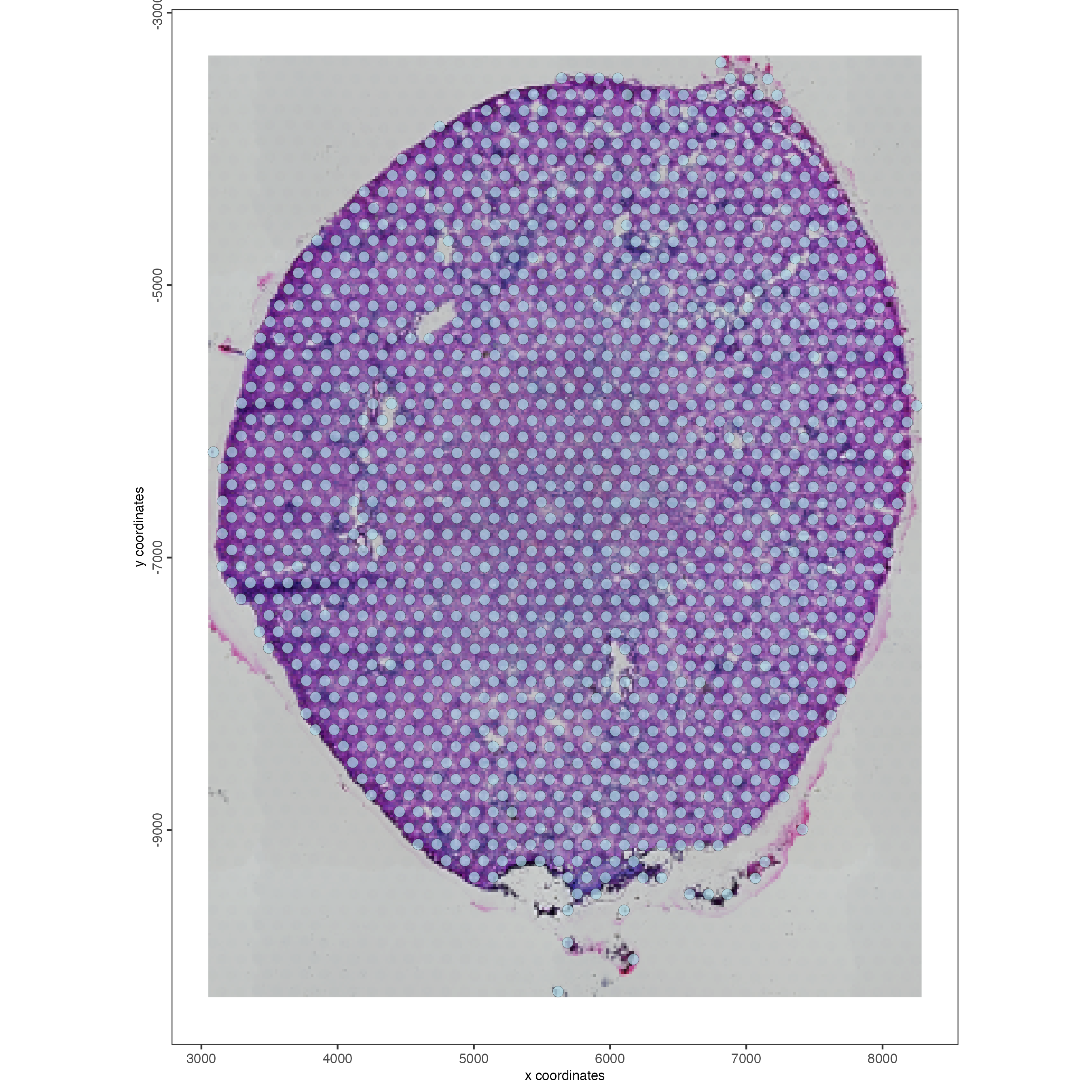
spatPlot2D(gobject = visium_kidney,
           show_image = TRUE,
           point_alpha = 0.7,
           cell_color = "nr_feats",
           color_as_factor = FALSE)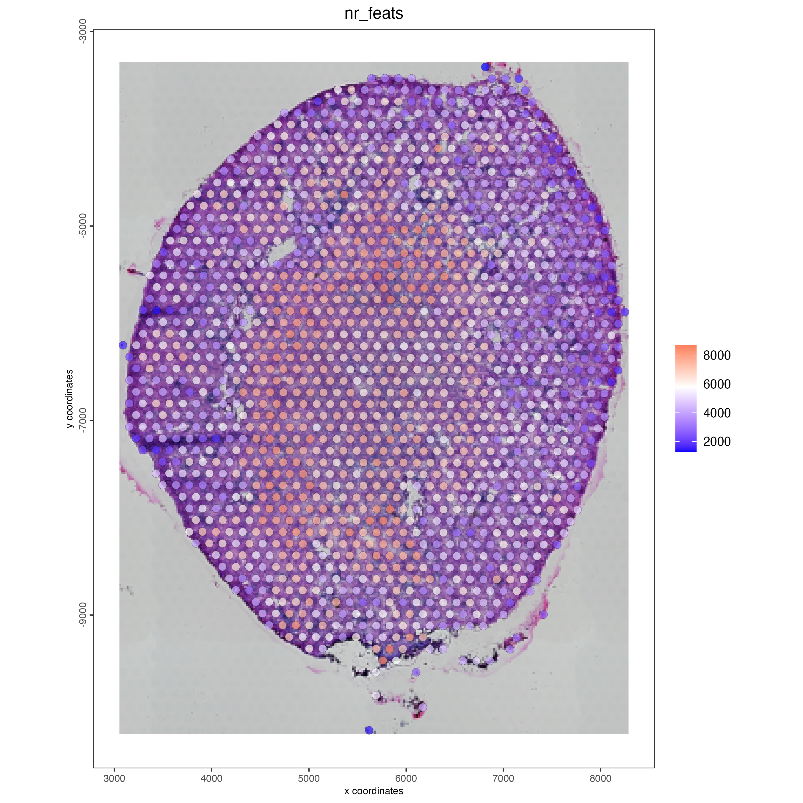
5 Dimension reduction
## highly variable features (genes)
visium_kidney <- calculateHVF(gobject = visium_kidney,
                              save_plot = TRUE)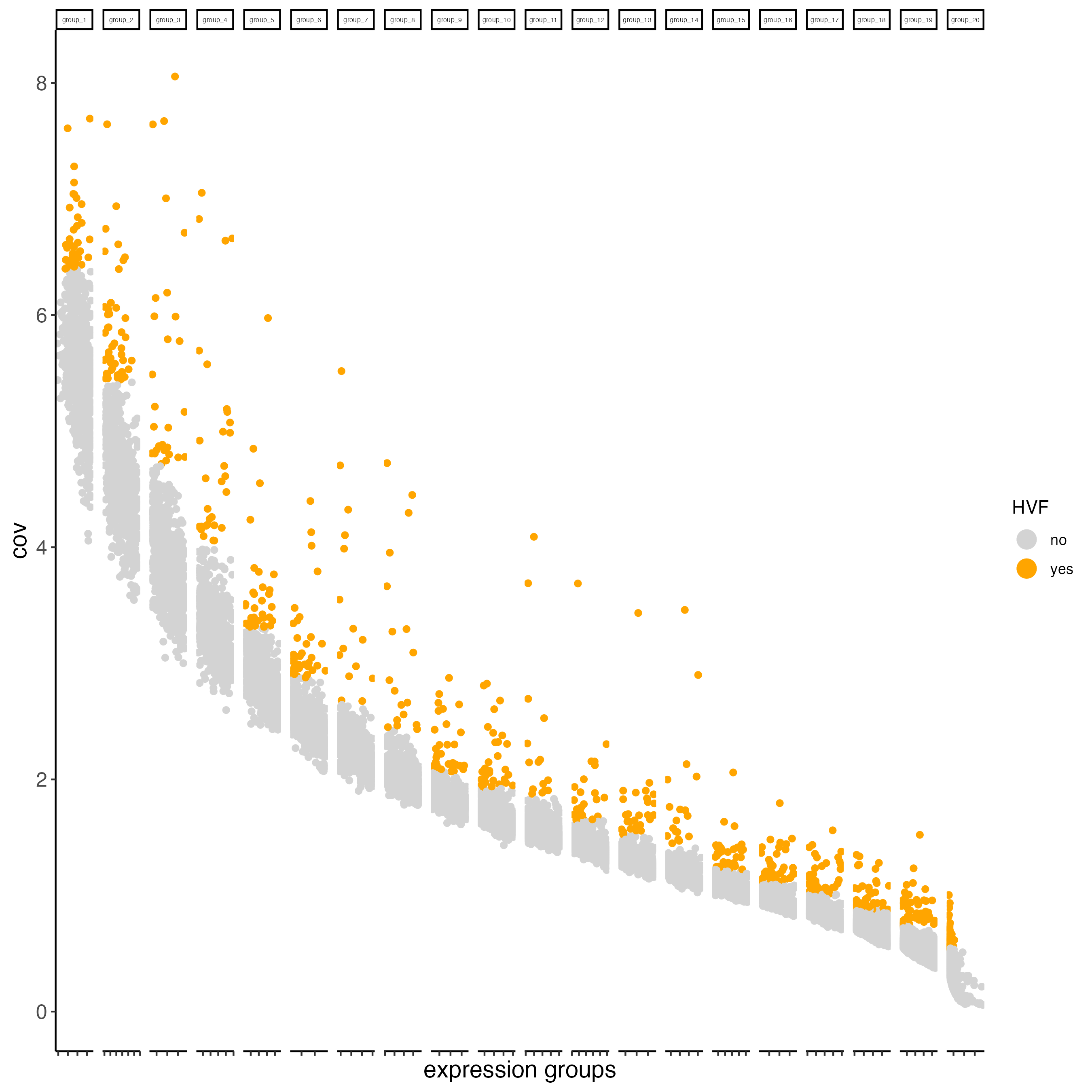
## run PCA on expression values (default)
visium_kidney <- runPCA(gobject = visium_kidney)

screePlot(visium_kidney,
          ncp = 30)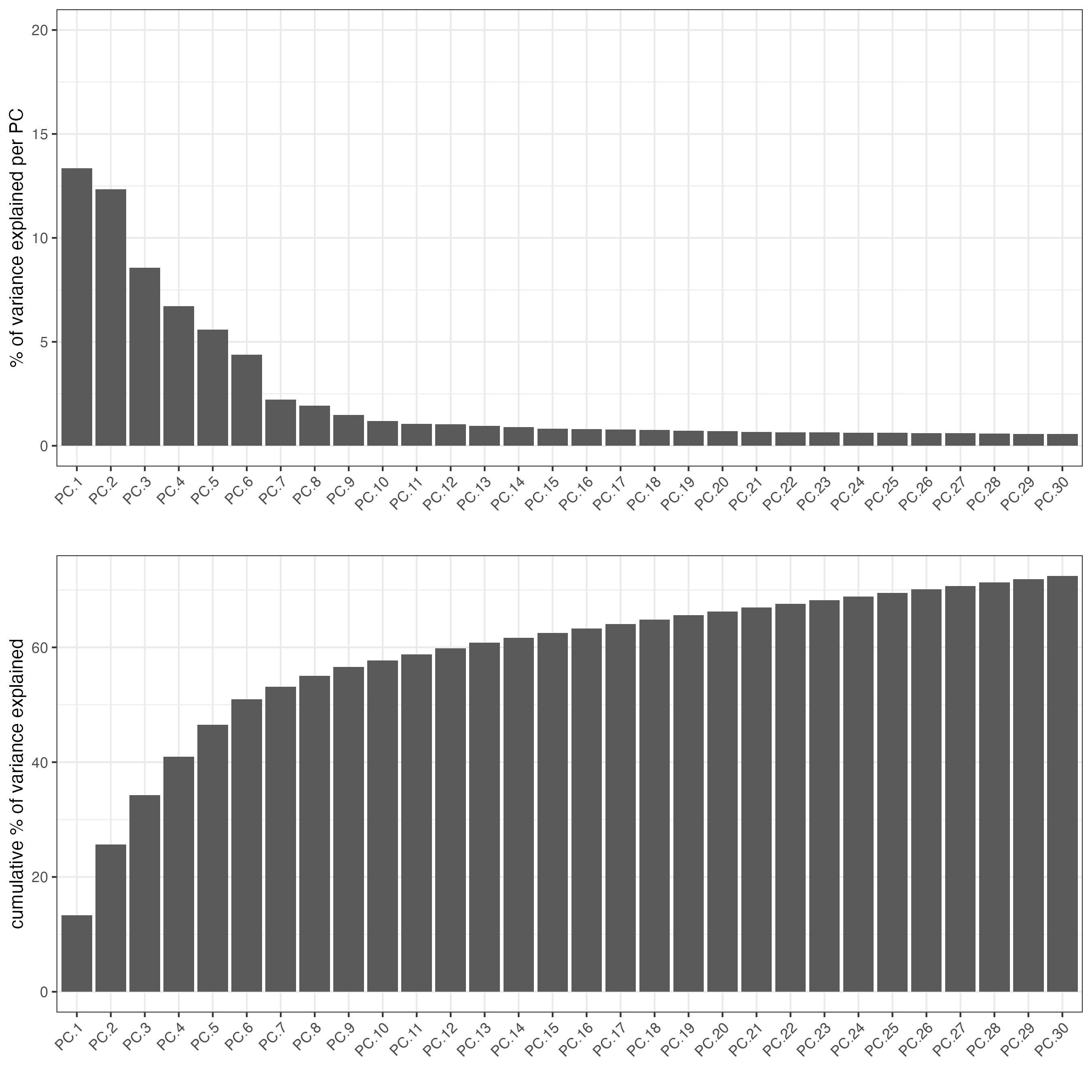
plotPCA(gobject = visium_kidney)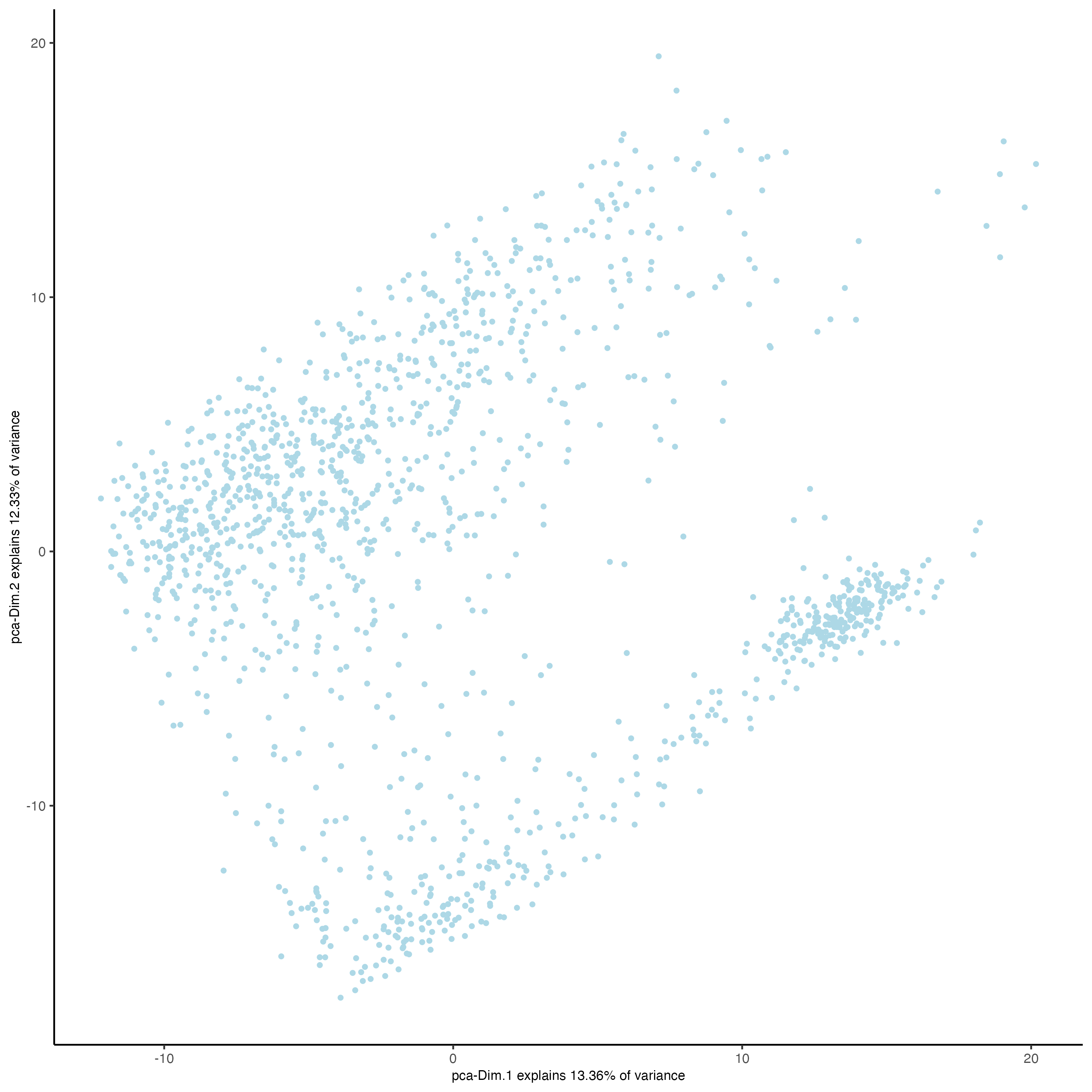
## run UMAP and tSNE on PCA space (default)
visium_kidney <- runUMAP(visium_kidney,
dimensions_to_use = 1:10)
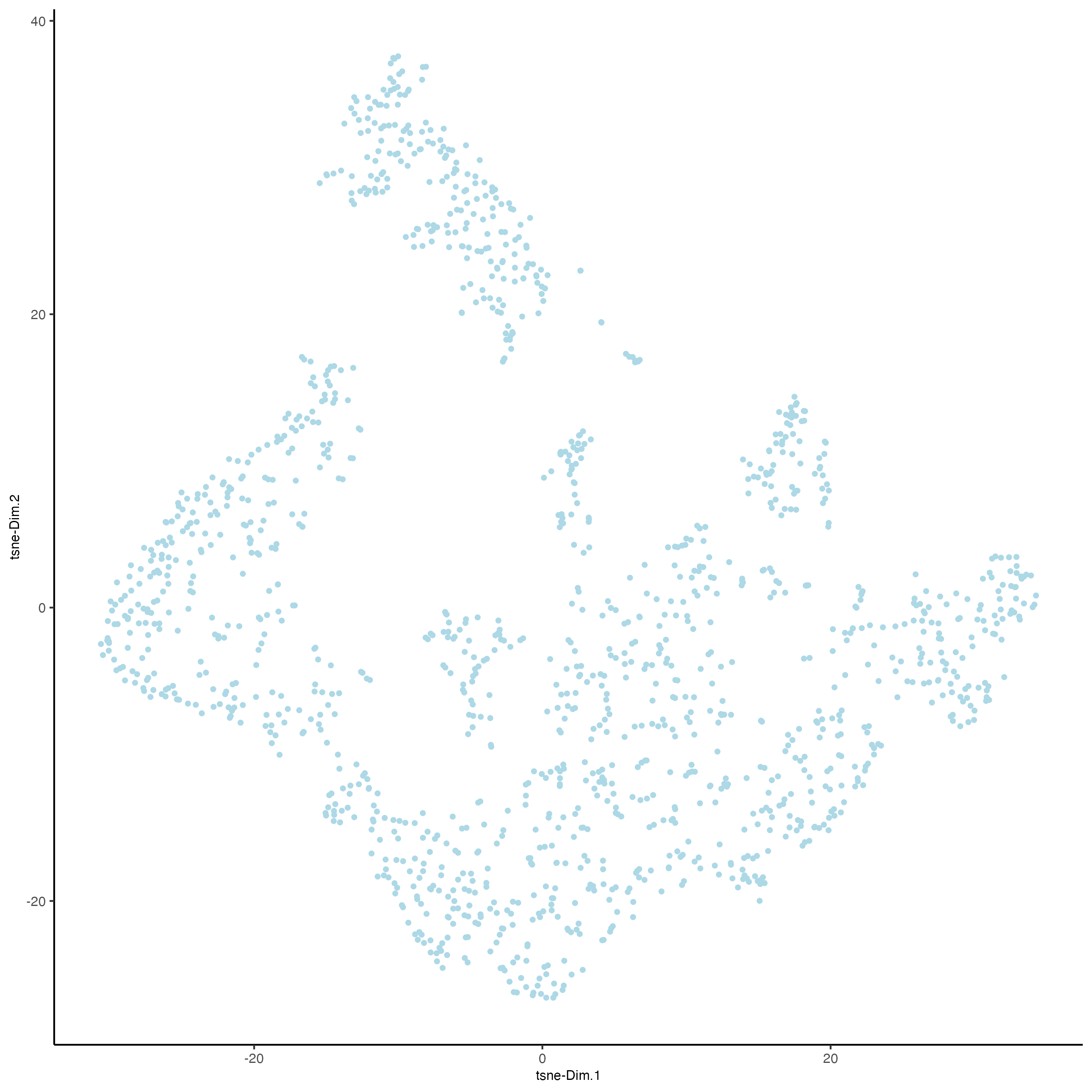
plotUMAP(gobject = visium_kidney)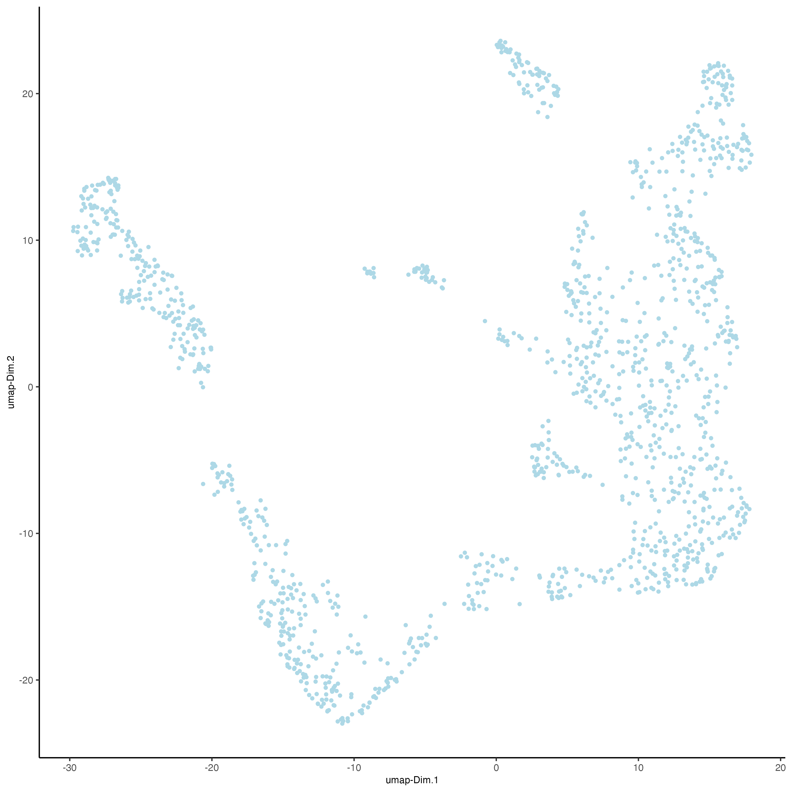
6 Clustering
## sNN network (default)
visium_kidney <- createNearestNetwork(gobject = visium_kidney,
                                      dimensions_to_use = 1:10,
                                      k = 15)

## Leiden clustering
visium_kidney <- doLeidenCluster(gobject = visium_kidney,
                                 resolution = 0.4,
                                 n_iterations = 1000)

plotUMAP(gobject = visium_kidney,
         cell_color = "leiden_clus",
         show_NN_network = TRUE,
         point_size = 2.5)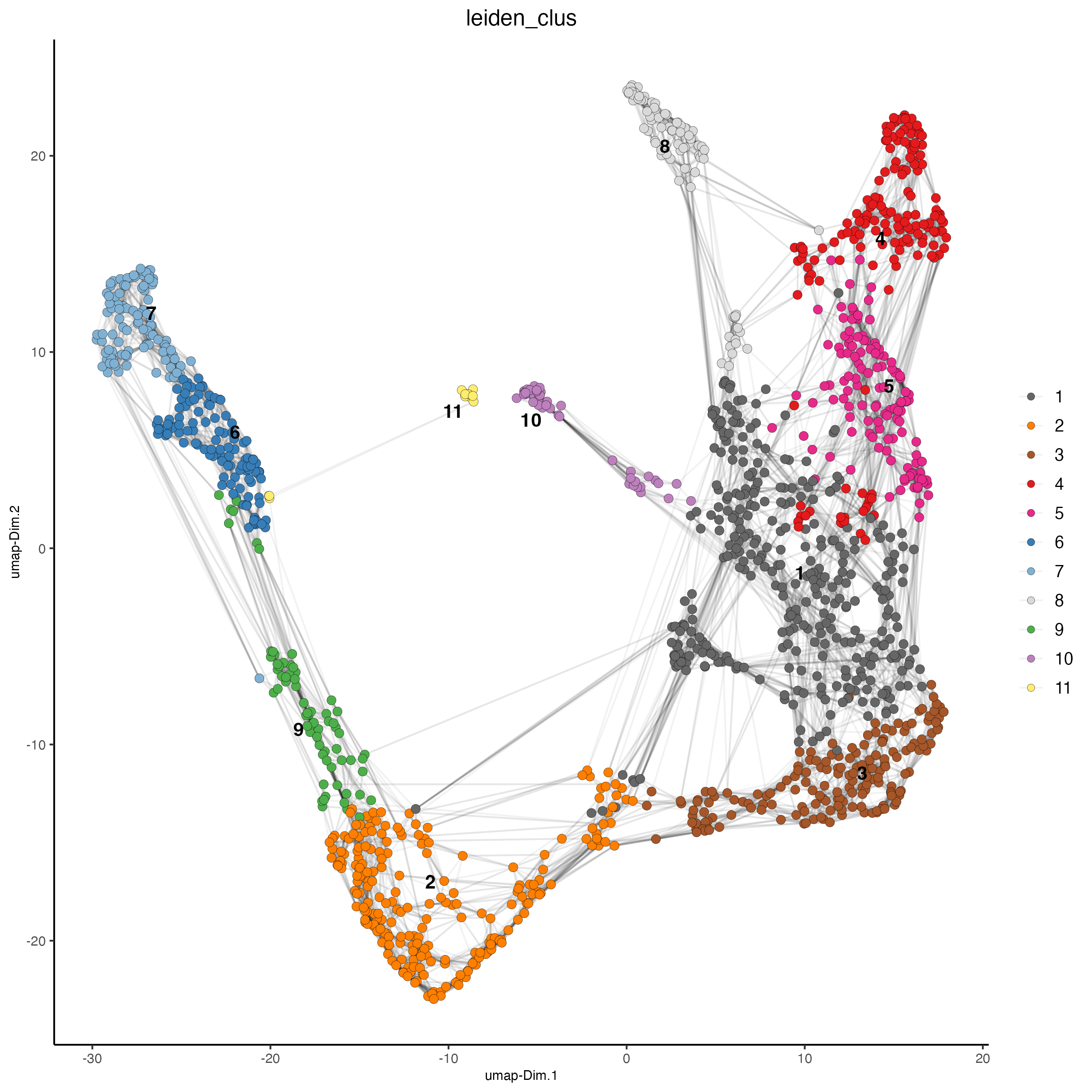
7 Co-visualize
# expression and spatial
spatDimPlot(gobject = visium_kidney,
            cell_color = "leiden_clus",
            dim_point_size = 2,
            spat_point_size = 2.5)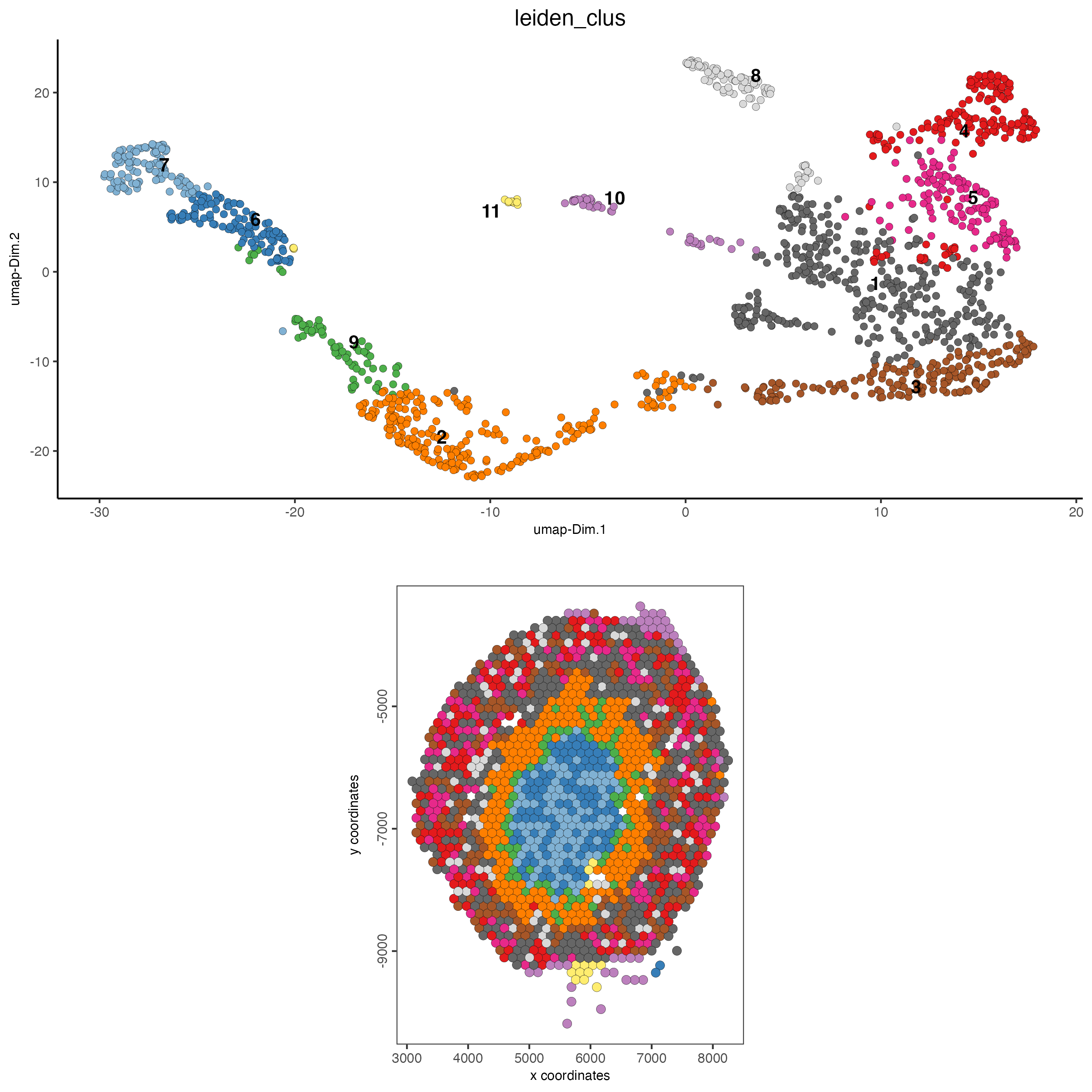
spatDimPlot(gobject = visium_kidney,
            cell_color = "nr_feats",
            color_as_factor = FALSE,
            dim_point_size = 2,
            spat_point_size = 2.5)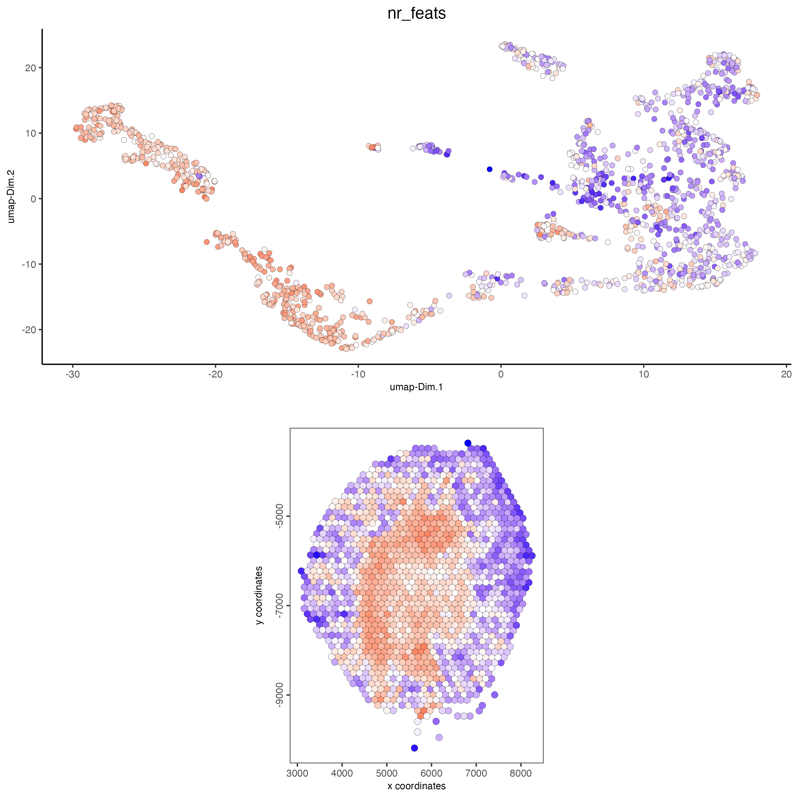
8 Cell type marker gene detection
8.1 gini
markers_gini <- findMarkers_one_vs_all(
    gobject = visium_kidney,
    method = "gini",
    expression_values = "normalized",
    cluster_column = "leiden_clus",
    min_featss = 20,
    min_expr_gini_score = 0.5,
    min_det_gini_score = 0.5
)

topgenes_gini <- markers_gini[, head(.SD, 2), by = "cluster"]$feats

# violinplot
violinPlot(visium_kidney,
           feats = unique(topgenes_gini),
           cluster_column = "leiden_clus",
           strip_text = 8,
           strip_position = "right")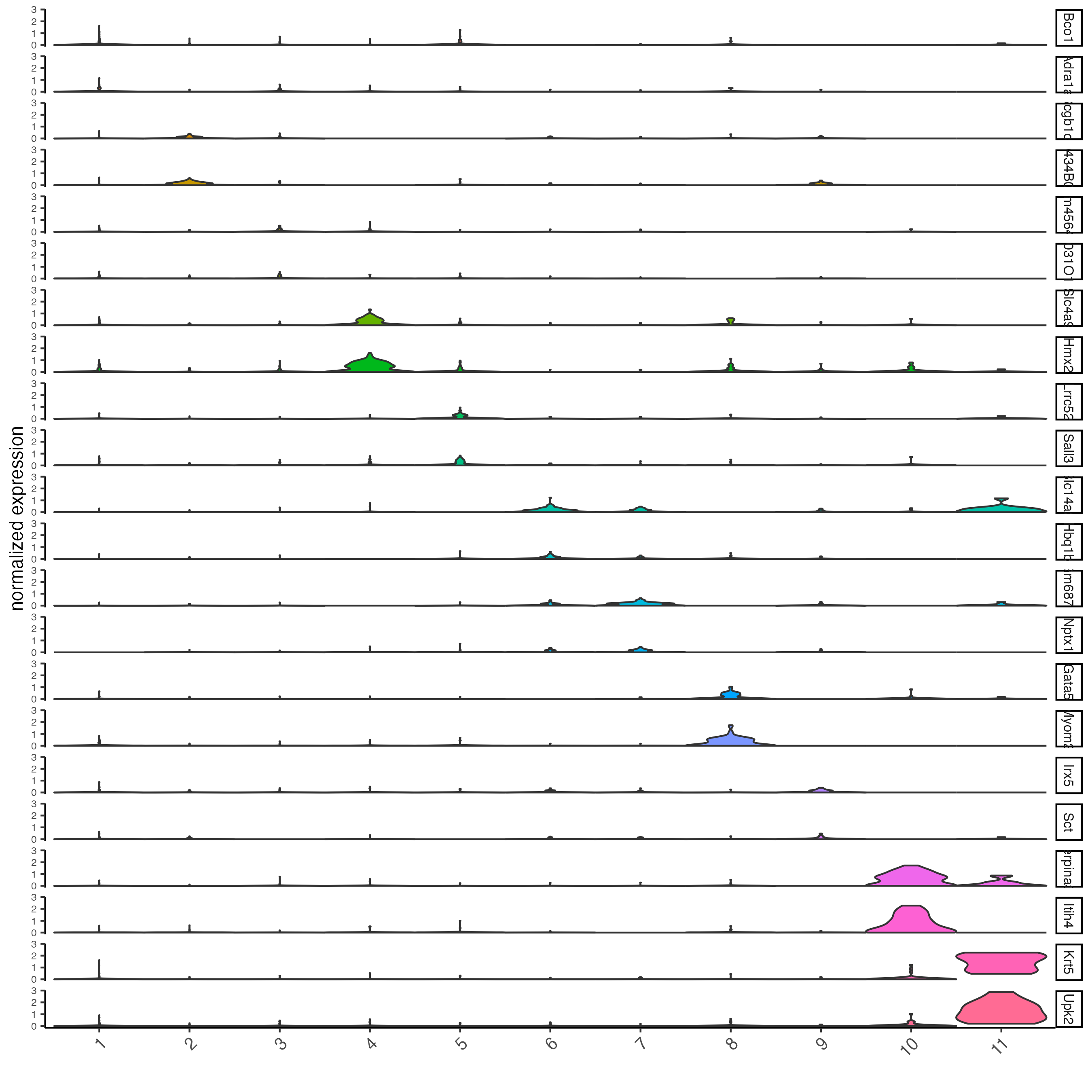
violinPlot(visium_kidney,
           feats = unique(topgenes_gini),
           cluster_column = "leiden_clus",
           strip_text = 8,
           strip_position = "right")
# cluster heatmap
plotMetaDataHeatmap(visium_kidney,
                    selected_feats = topgenes_gini,
                    metadata_cols = "leiden_clus",
                    x_text_size = 10,
                    y_text_size = 10)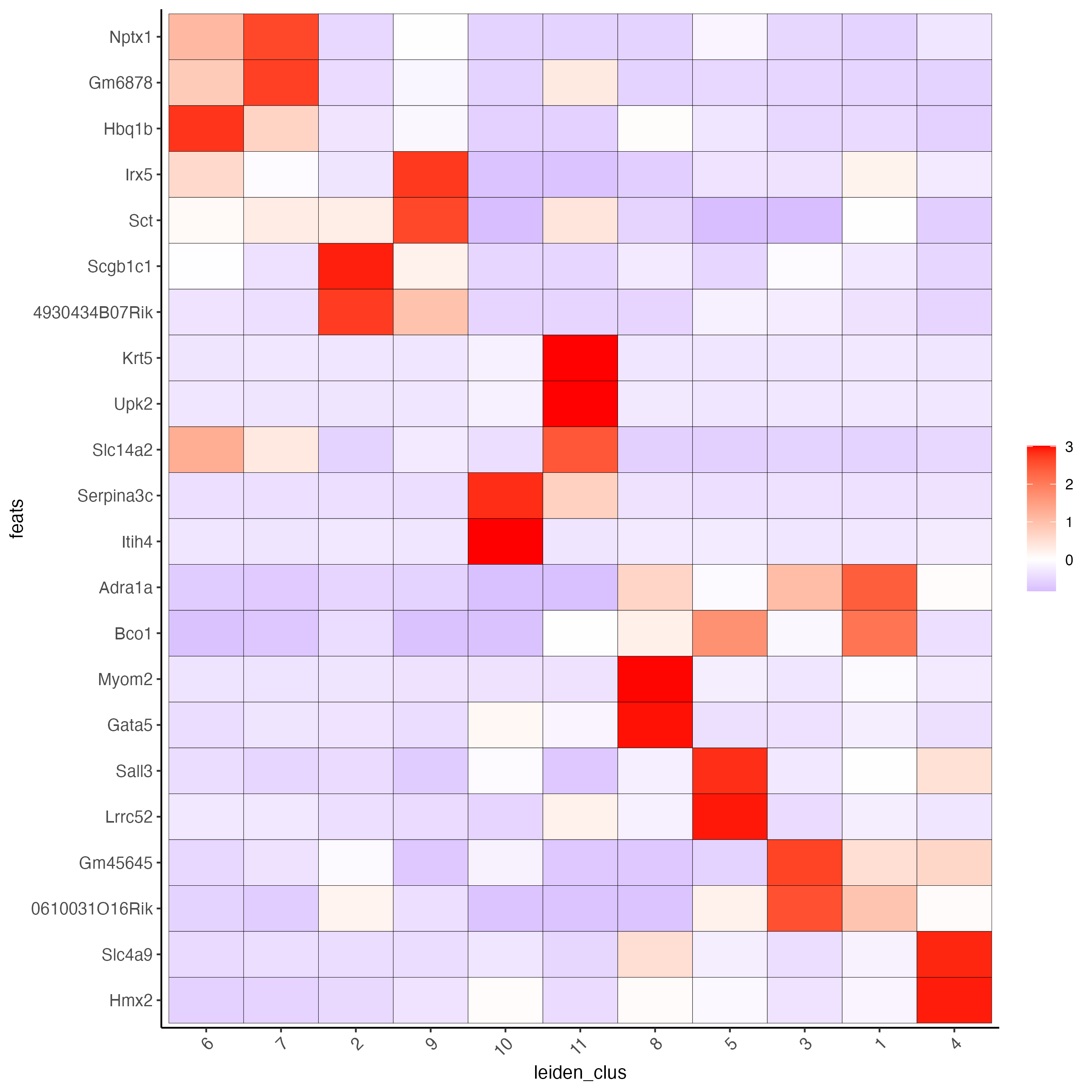
# umap plots
dimFeatPlot2D(visium_kidney,
              expression_values = "scaled",
              feats = markers_gini[, head(.SD, 1), by = "cluster"]$feats,
              cow_n_col = 3,
              point_size = 1)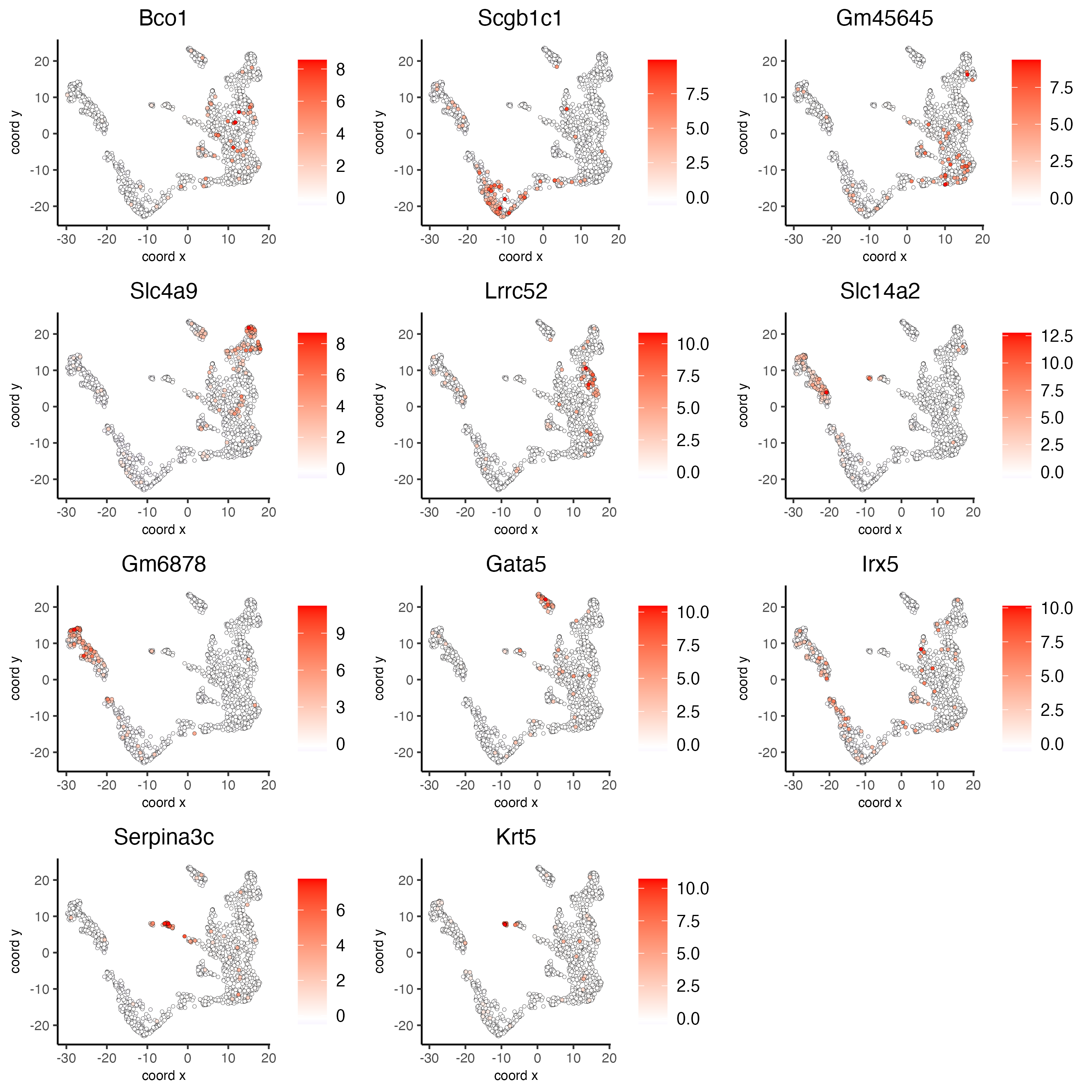
8.2 Scran
markers_scran <- findMarkers_one_vs_all(
    gobject = visium_kidney,
    method = "scran",
    expression_values = "normalized",
    cluster_column = "leiden_clus"
)

topgenes_scran <- markers_scran[, head(.SD, 2), by = "cluster"]$feats

violinPlot(visium_kidney,
           feats = unique(topgenes_scran),
           cluster_column = "leiden_clus",
           strip_text = 10,
           strip_position = "right")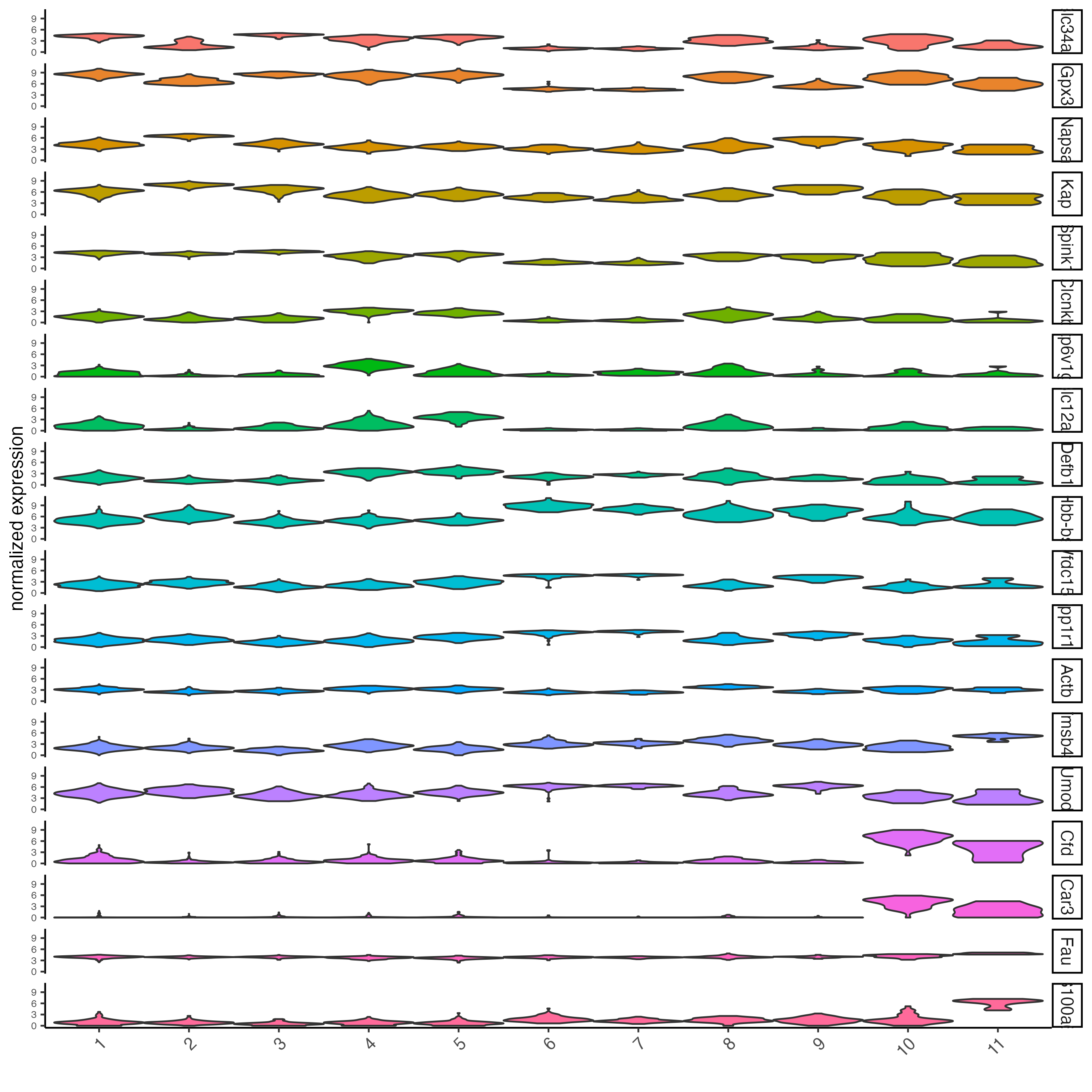
# cluster heatmap
plotMetaDataHeatmap(visium_kidney,
                    selected_feats = topgenes_scran,
                    metadata_cols = "leiden_clus")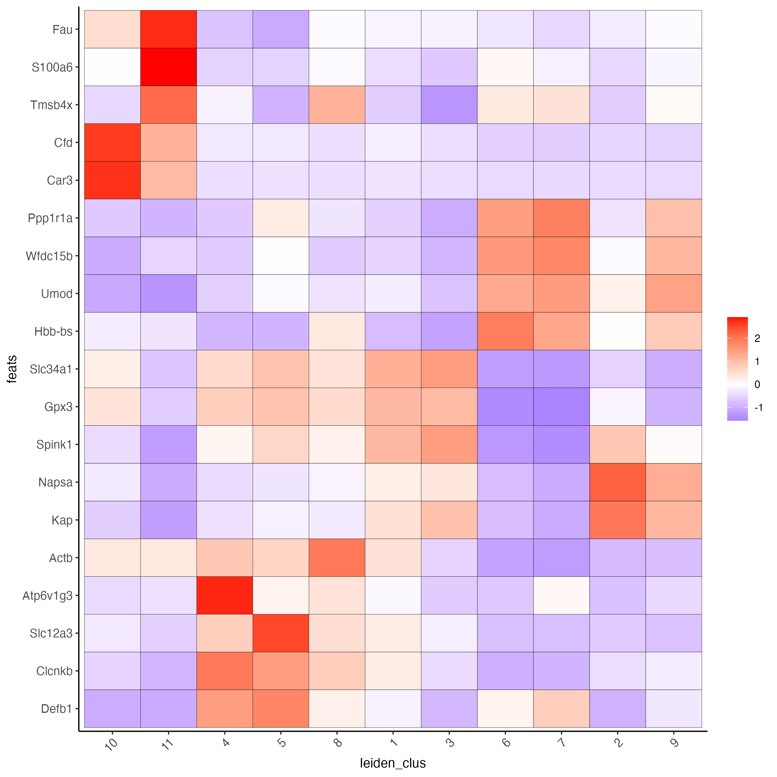
# umap plots
dimFeatPlot2D(visium_kidney,
              expression_values = "scaled",
              feats = markers_scran[, head(.SD, 1), by = "cluster"]$feats,
              cow_n_col = 3,
              point_size = 1)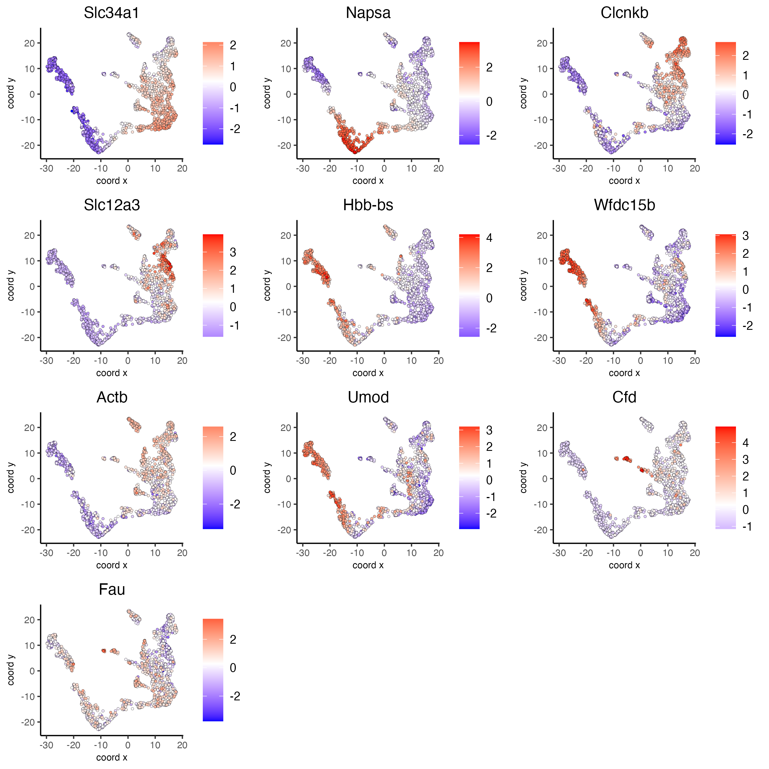
9 Cell-type annotation
Visium spatial transcriptomics does not provide single-cell resolution, making cell type annotation a harder problem. Giotto provides 3 ways to calculate enrichment of specific cell-type signature gene list:
- PAGE
- rank
- hypergeometric test
10 Spatial grid
visium_kidney <- createSpatialGrid(
    gobject = visium_kidney,
    sdimx_stepsize = 400,
    sdimy_stepsize = 400,
    minimum_padding = 0
)

spatPlot(visium_kidney,
         cell_color = "leiden_clus",
         show_grid = TRUE,
         grid_color = "red",
         spatial_grid_name = "spatial_grid")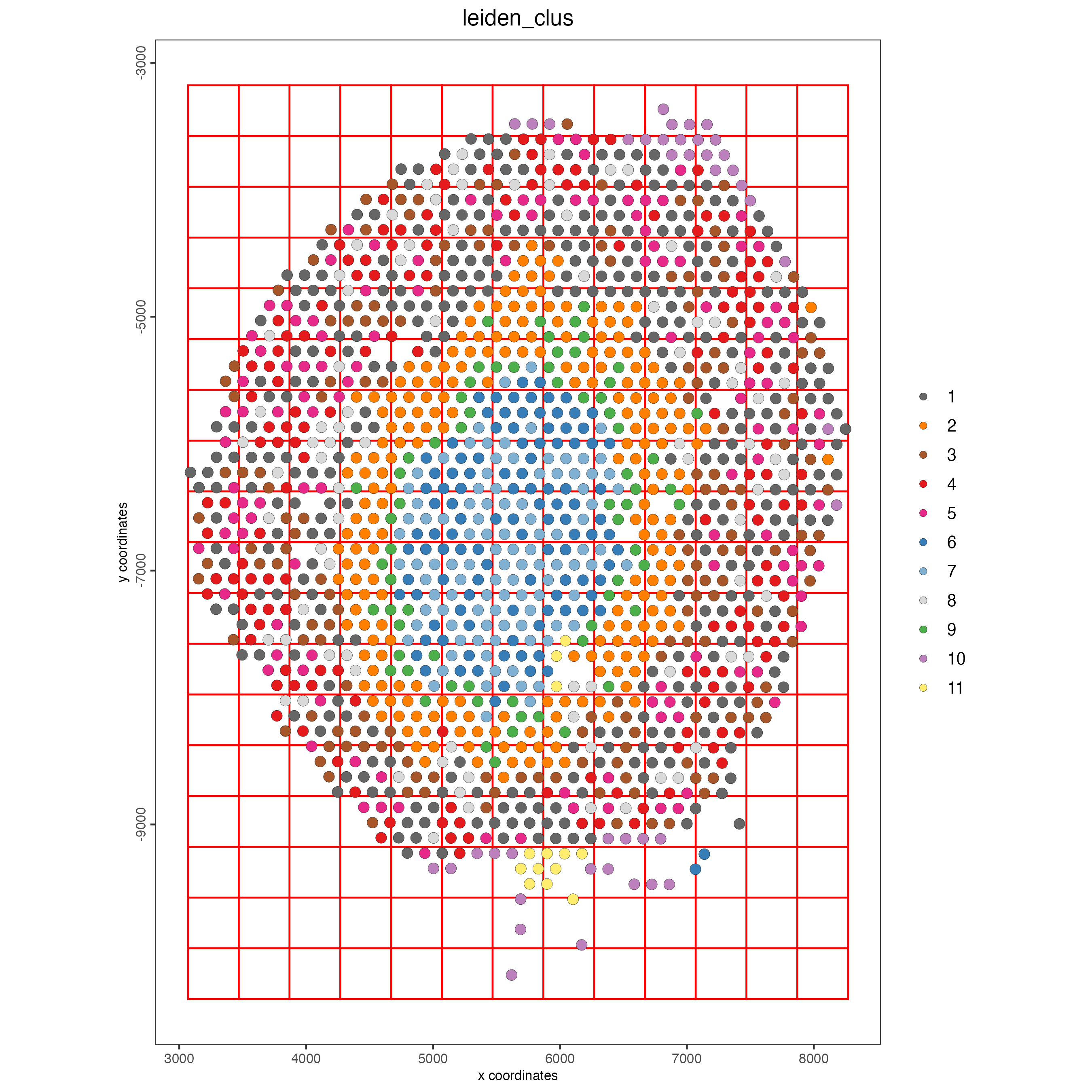
11 Spatial network
## delaunay network: stats + creation
plotStatDelaunayNetwork(gobject = visium_kidney,
                        maximum_distance = 400)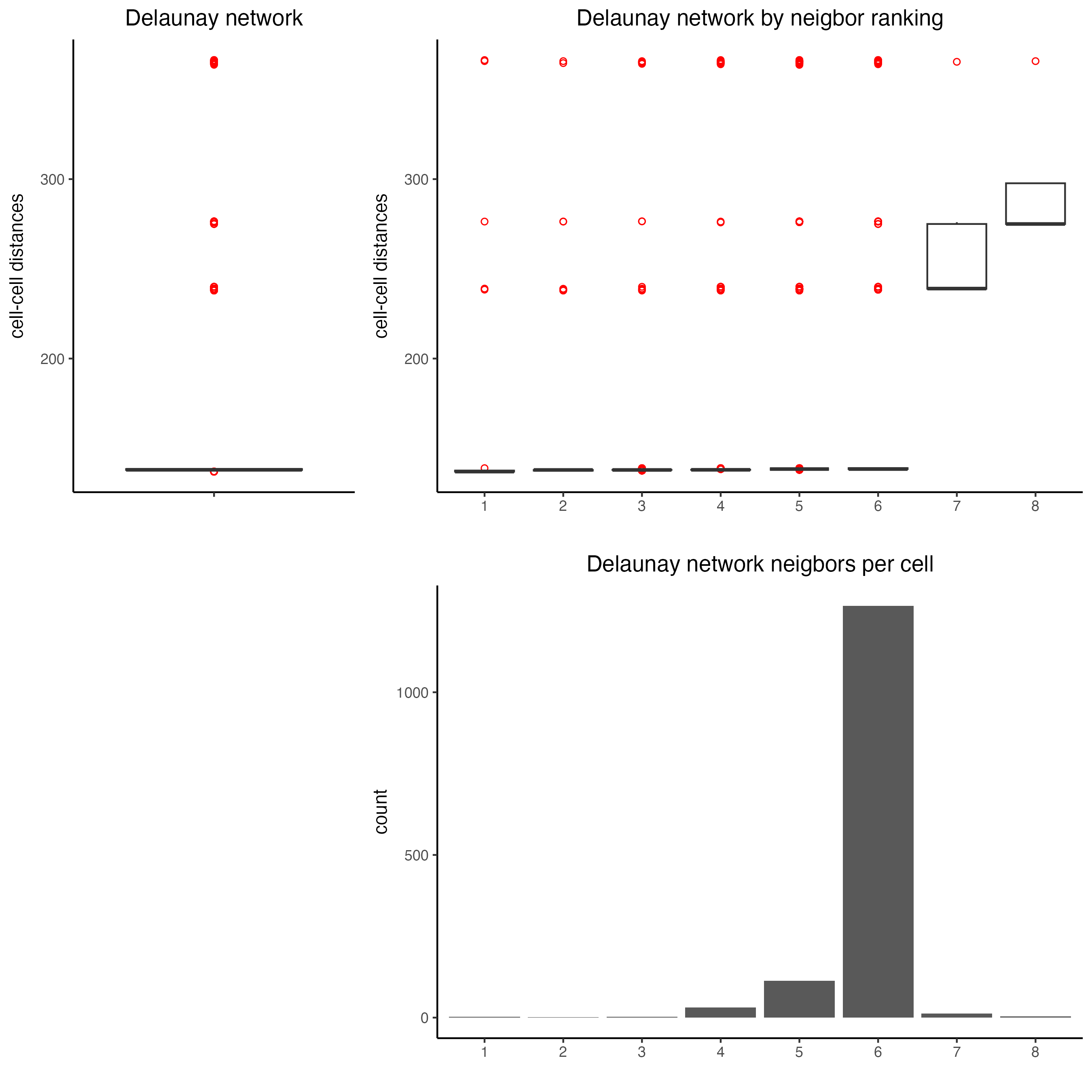
visium_kidney <- createSpatialNetwork(gobject = visium_kidney,
                                      minimum_k = 0)

showNetworks(visium_kidney)

spatPlot(gobject = visium_kidney,
         show_network = TRUE,
         network_color = "blue",
         spatial_network_name = "Delaunay_network")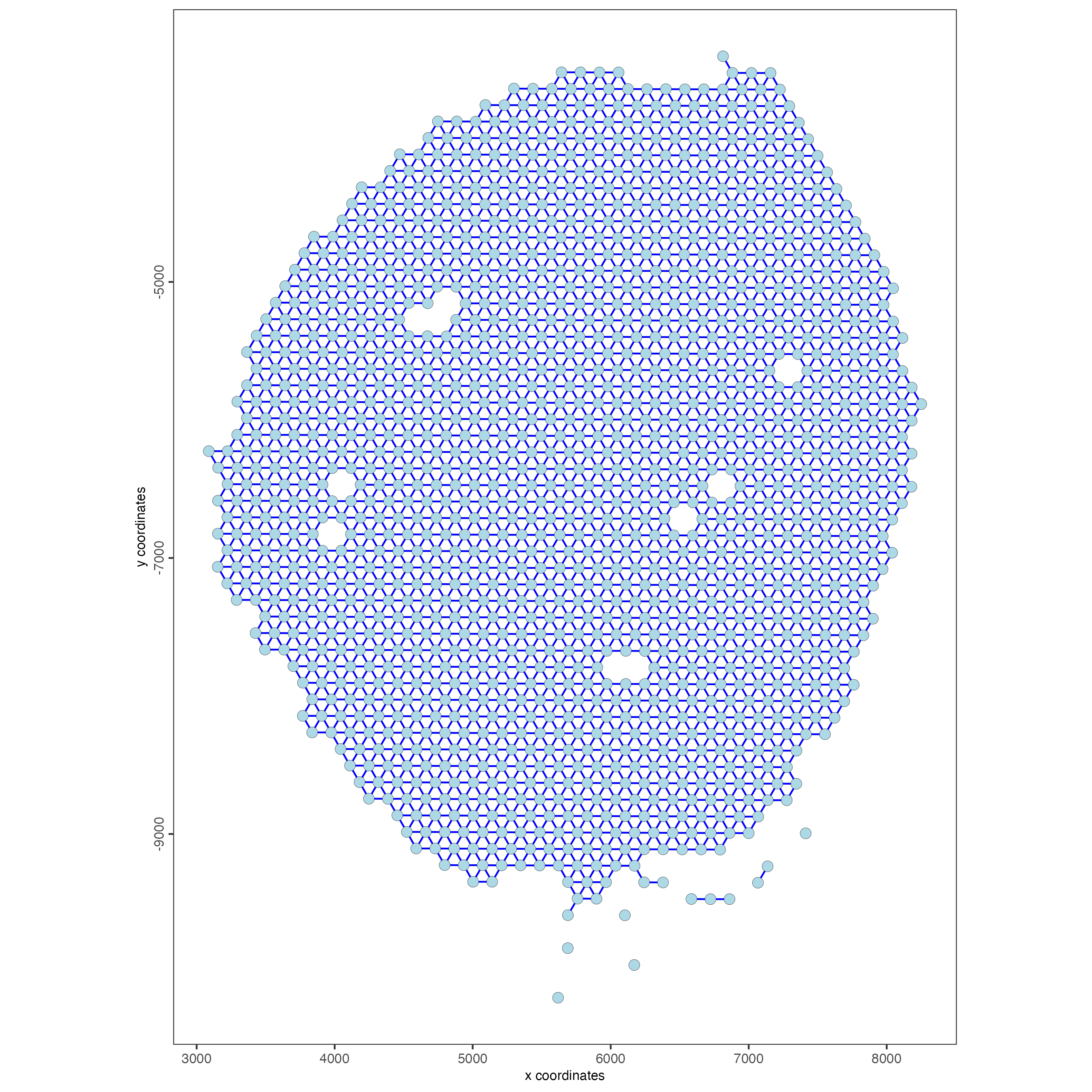
12 Spatial genes
12.1 Spatial genes
## kmeans binarization
km_spatialfeats <- binSpect(visium_kidney)

spatFeatPlot2D(visium_kidney,
               expression_values = "scaled",
               feats = km_spatialfeats$feats[1:6],
               cow_n_col = 2,
               point_size = 1.5)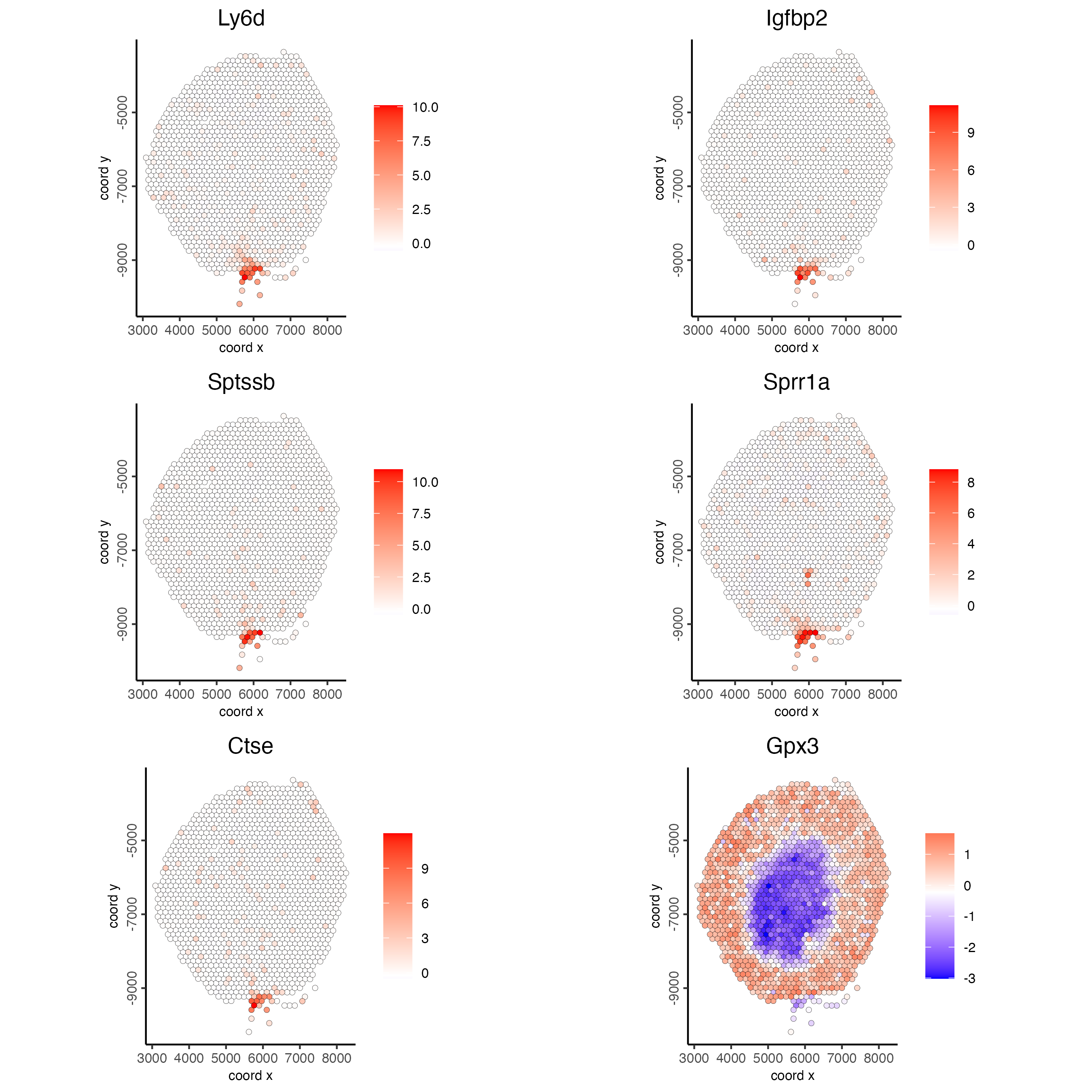
## rank binarization
ranktest <- binSpect(visium_kidney,
                     bin_method = "rank")

spatFeatPlot2D(visium_kidney,
               expression_values = "scaled",
               feats = ranktest$feats[1:6],
               cow_n_col = 2,
               point_size = 1.5)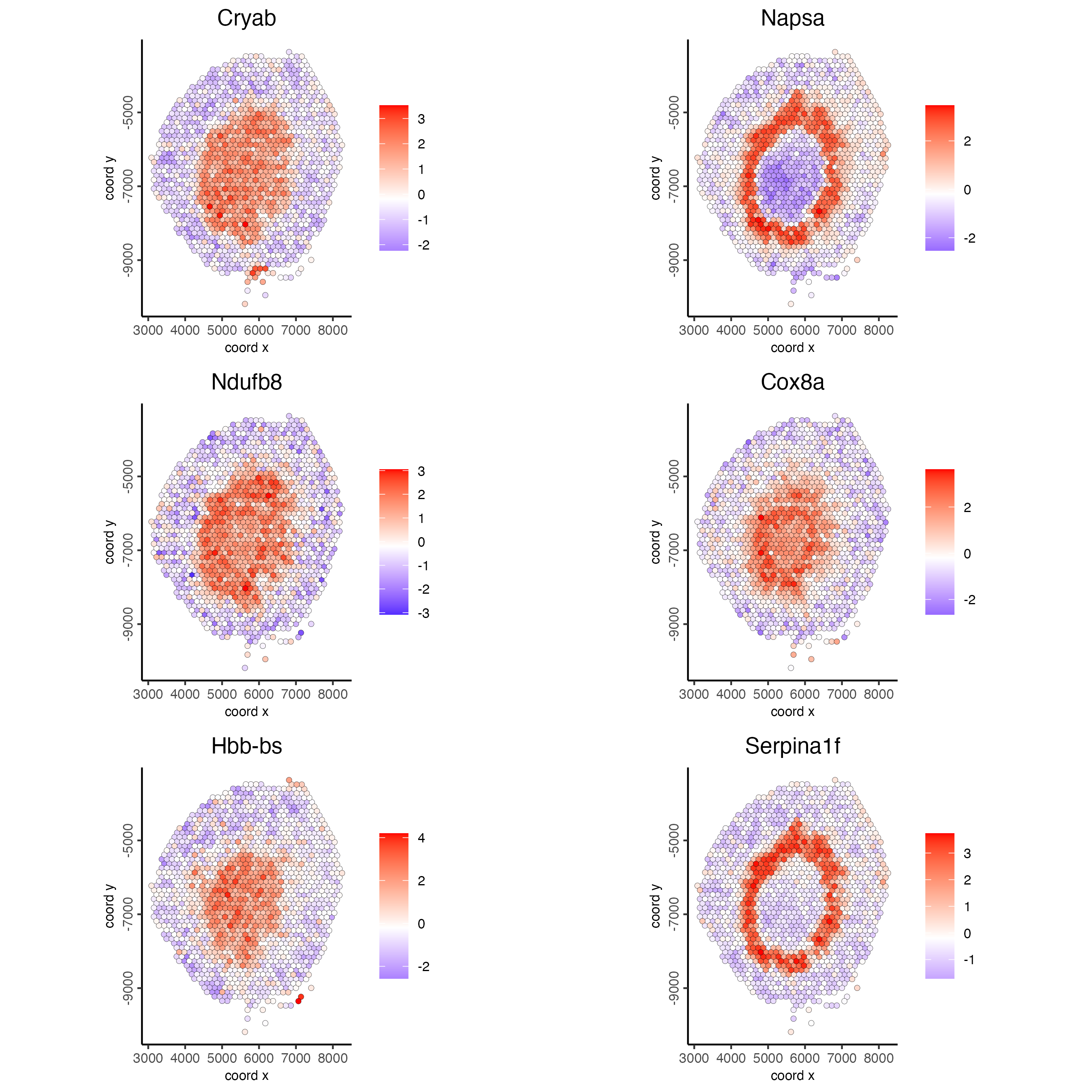
12.2 Spatial co-expression patterns
## spatially correlated genes ##
my_spatial_genes <- km_spatialfeats[1:500]$feats

# 1. calculate gene spatial correlation and single-cell correlation
# create spatial correlation object
spat_cor_netw_DT <- detectSpatialCorFeats(
  visium_kidney,
  method = "network",
  spatial_network_name = "Delaunay_network",
  subset_feats = my_spatial_genes
)

# 2. identify most similar spatially correlated genes for one gene
top10_genes <- showSpatialCorFeats(spat_cor_netw_DT,
                                   feats = "Napsa",
                                   show_top_feats = 10)

spatFeatPlot2D(visium_kidney,
               expression_values = "scaled",
               feats = c("Napsa", "Kap", "Defb29", "Prdx1"),
               point_size = 3)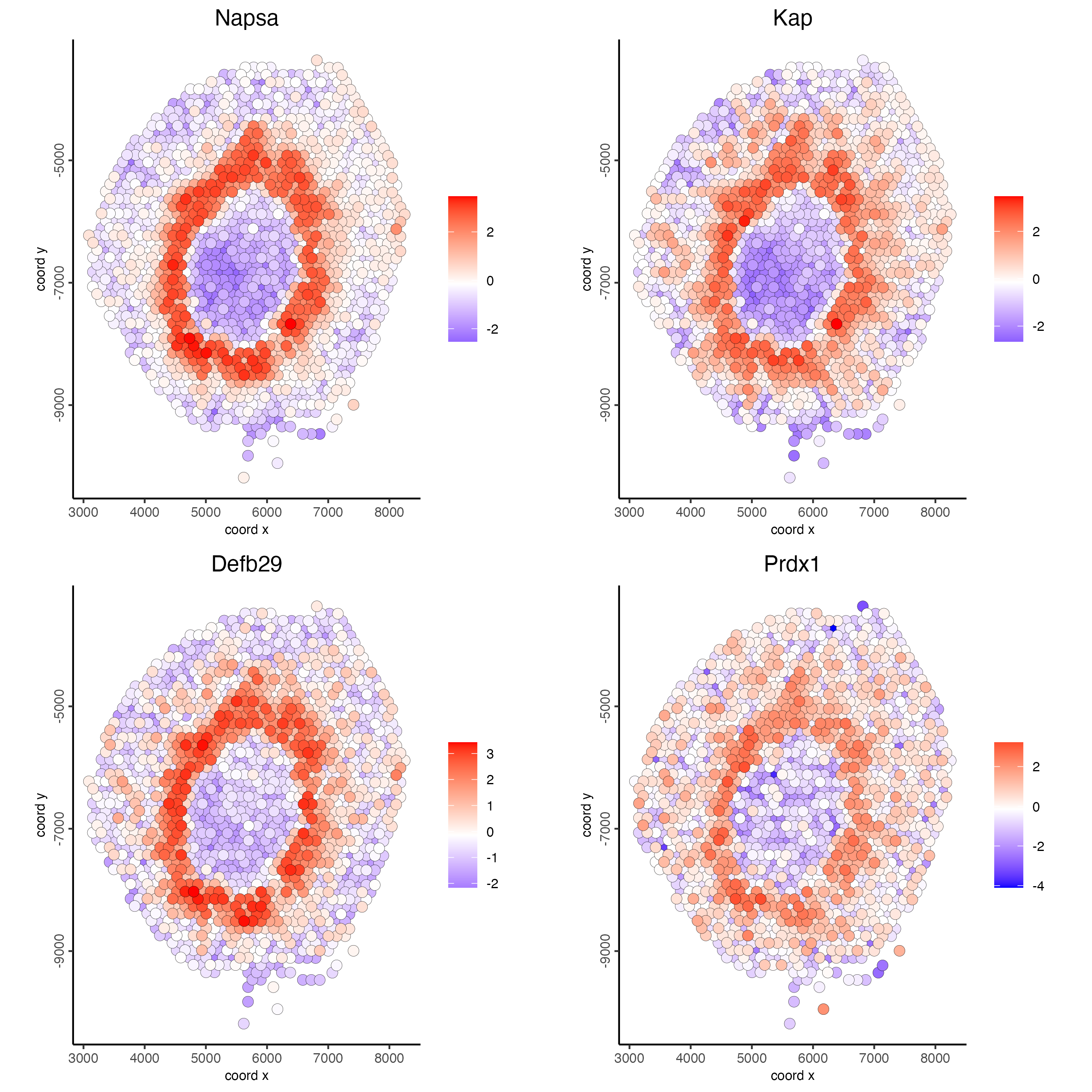
# 3. cluster correlated genes & visualize
spat_cor_netw_DT <- clusterSpatialCorFeats(spat_cor_netw_DT,
                                           name = "spat_netw_clus",
                                           k = 8)

heatmSpatialCorFeats(visium_kidney,
                     spatCorObject = spat_cor_netw_DT,
                     use_clus_name = "spat_netw_clus",
                     heatmap_legend_param = list(title = NULL))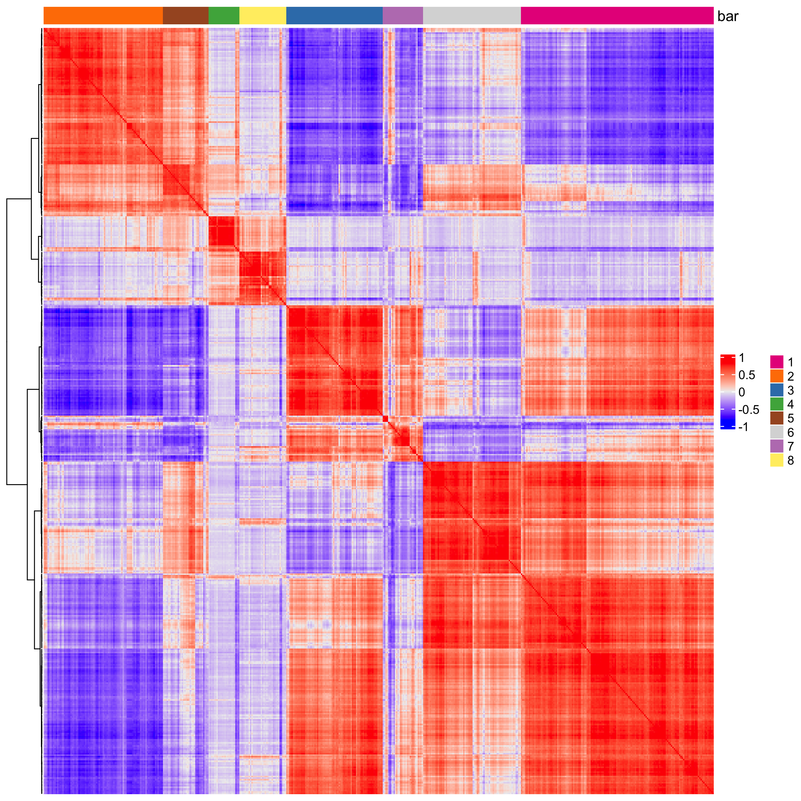
# 4. rank spatial correlated clusters and show genes for selected clusters
netw_ranks <- rankSpatialCorGroups(visium_kidney,
                                   spatCorObject = spat_cor_netw_DT,
                                   use_clus_name = "spat_netw_clus")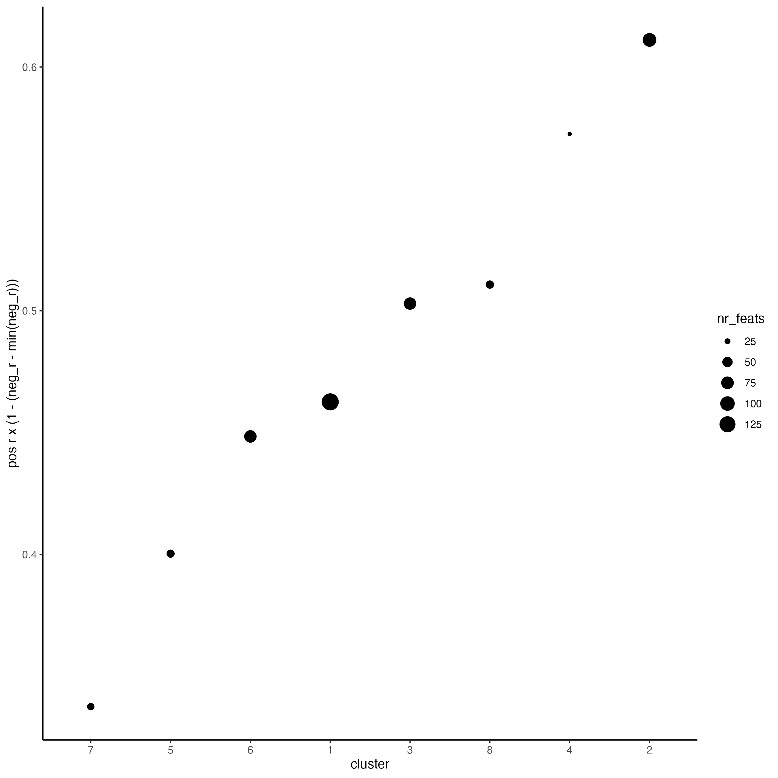
top_netw_spat_cluster <- showSpatialCorFeats(spat_cor_netw_DT,
                                             use_clus_name = "spat_netw_clus",
                                             selected_clusters = 6,
                                             show_top_feats = 1)

# 5. create metagene enrichment score for clusters
cluster_genes_DT <- showSpatialCorFeats(spat_cor_netw_DT,
                                        use_clus_name = "spat_netw_clus",
                                        show_top_feats = 1)

cluster_genes <- cluster_genes_DT$clus
names(cluster_genes) <- cluster_genes_DT$feat_ID

visium_kidney <- createMetafeats(visium_kidney,
                                 feat_clusters = cluster_genes,
                                 name = "cluster_metagene")

showGiottoSpatEnrichments(visium_kidney)

spatCellPlot(visium_kidney,
             spat_enr_names = "cluster_metagene",
             cell_annotation_values = netw_ranks$clusters,
             point_size = 1.5,
             cow_n_col = 4)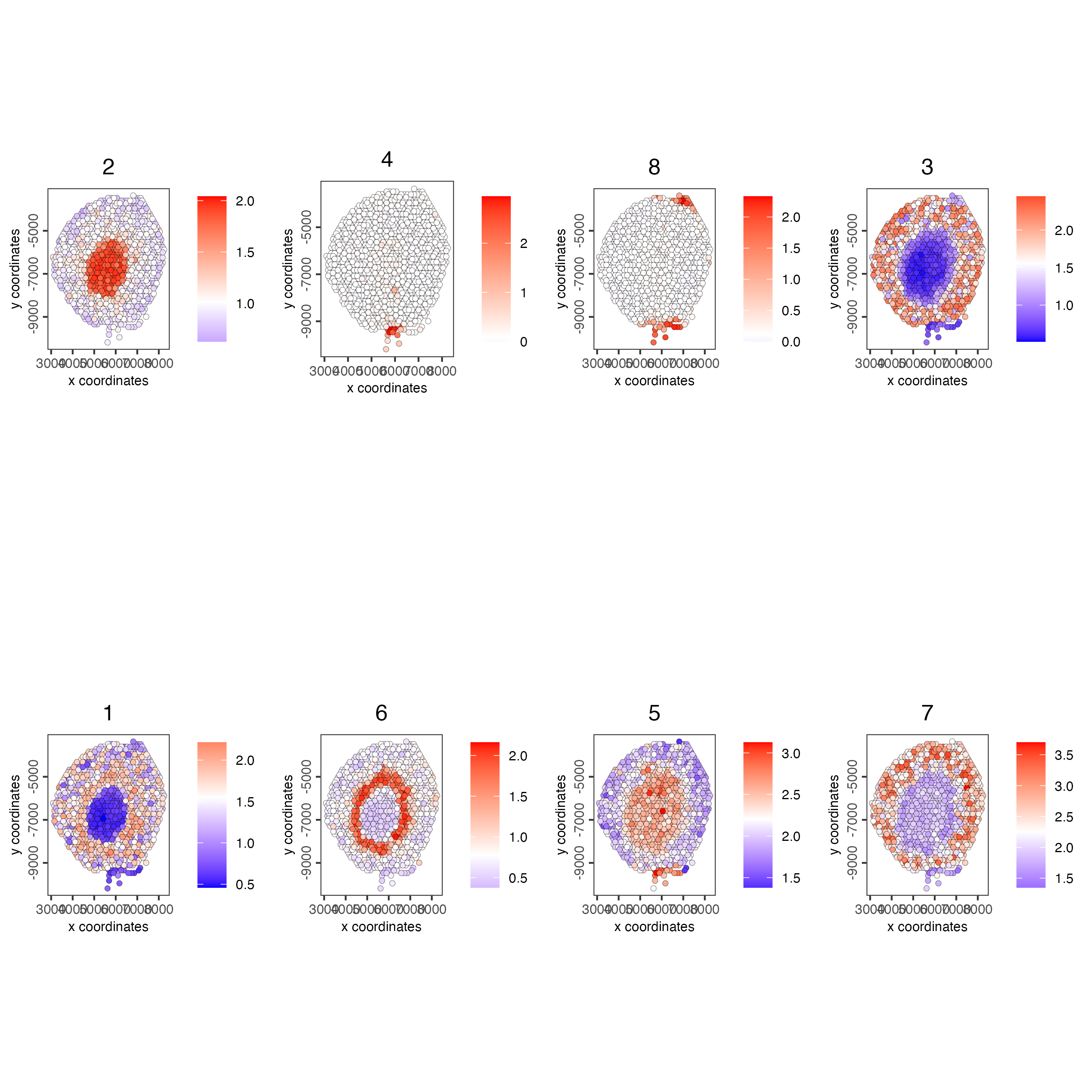
13 HMRF domains
# HMRF requires a fully connected network!
visium_kidney <- createSpatialNetwork(gobject = visium_kidney,
                                      minimum_k = 2,
                                      name = "Delaunay_full")

# spatial genes
my_spatial_genes <- km_spatialfeats[1:100]$feats

# do HMRF with different betas
hmrf_folder <- file.path(data_path, "HMRF_results")
if (!file.exists(hmrf_folder)) dir.create(hmrf_folder, recursive = TRUE)

# if Rscript is not found, you might have to create a symbolic link, e.g.
# cd /usr/local/bin
# sudo ln -s /Library/Frameworks/R.framework/Resources/Rscript Rscript
HMRF_spatial_genes <- doHMRF(
    gobject = visium_kidney,
    expression_values = "scaled",
    spatial_network_name = "Delaunay_full",
    spatial_genes = my_spatial_genes,
    k = 5,
    betas = c(0, 1, 6),
    output_folder = file.path(hmrf_folder, "Spatial_genes/SG_topgenes_k5_scaled"))
## alternative way to view HMRF results
# results = writeHMRFresults(gobject = ST_test,
#                           HMRFoutput = HMRF_spatial_genes,
#                           k = 5, betas_to_view = seq(0, 25, by = 5))
# ST_test = addCellMetadata(ST_test, new_metadata = results, by_column = T, column_cell_ID = 'cell_ID')


## add HMRF of interest to giotto object
visium_kidney <- addHMRF(gobject = visium_kidney,
                         HMRFoutput = HMRF_spatial_genes,
                         k = 5,
                         betas_to_add = c(0, 2),
                         hmrf_name = "HMRF")

## visualize
spatPlot(gobject = visium_kidney,
         cell_color = "HMRF_k5_b.0",
         point_size = 5)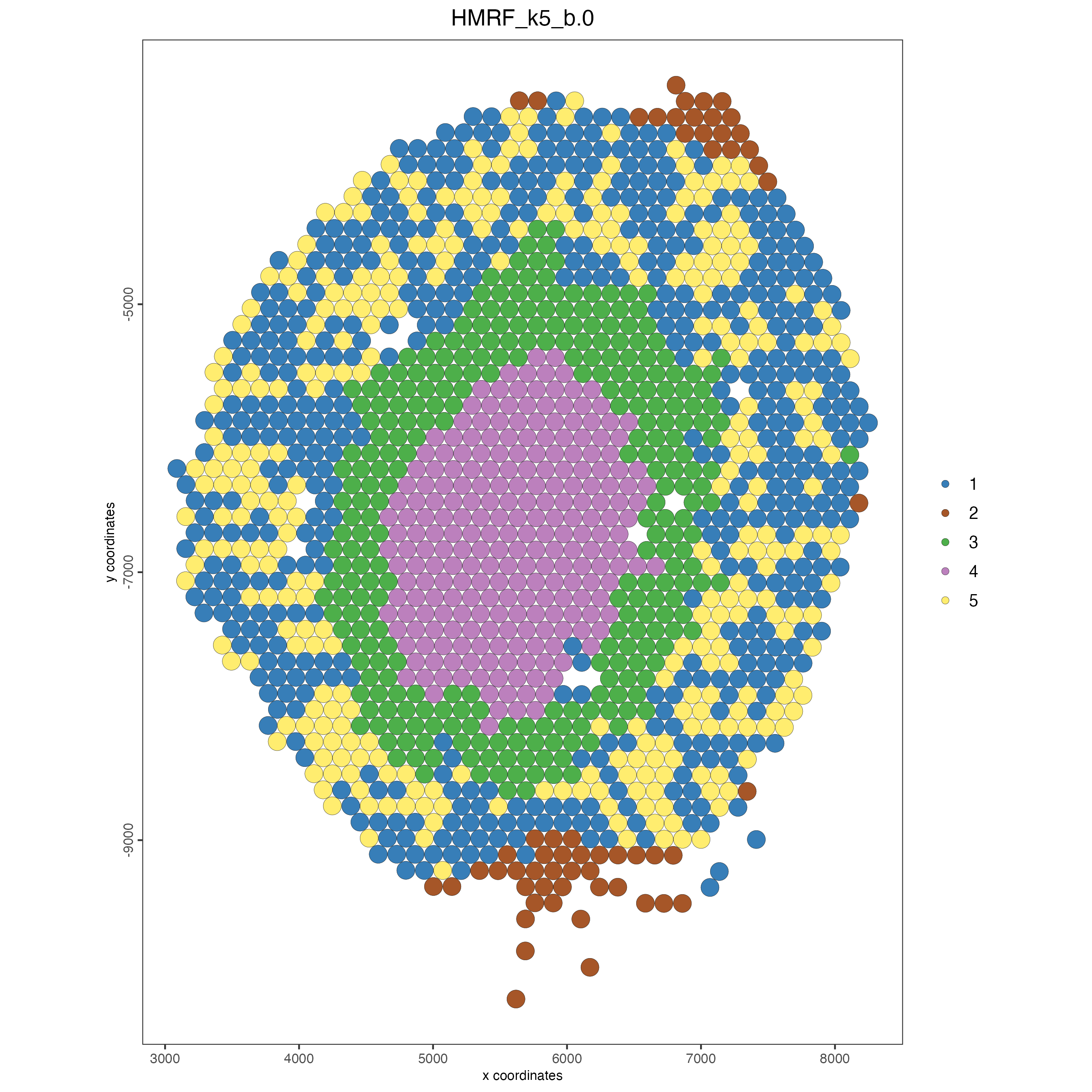
spatPlot(gobject = visium_kidney,
         cell_color = "HMRF_k5_b.2",
         point_size = 5)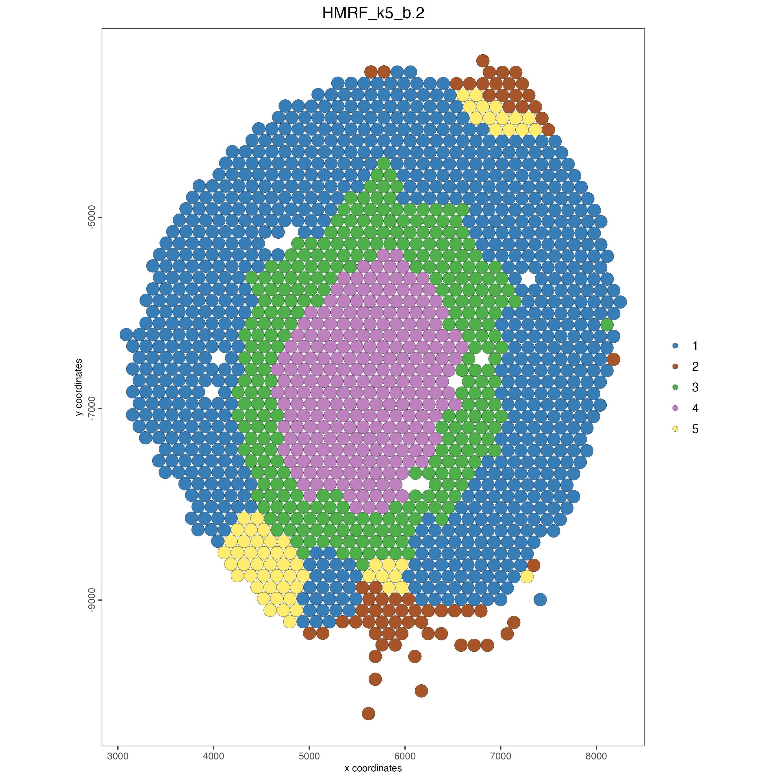
14 Session info
R version 4.4.0 (2024-04-24)
Platform: x86_64-apple-darwin20
Running under: macOS Sonoma 14.6.1

Matrix products: default
BLAS:   /System/Library/Frameworks/Accelerate.framework/Versions/A/Frameworks/vecLib.framework/Versions/A/libBLAS.dylib
LAPACK: /Library/Frameworks/R.framework/Versions/4.4-x86_64/Resources/lib/libRlapack.dylib;  LAPACK version 3.12.0

locale:
[1] en_US.UTF-8/en_US.UTF-8/en_US.UTF-8/C/en_US.UTF-8/en_US.UTF-8

time zone: America/New_York
tzcode source: internal

attached base packages:
[1] stats     graphics  grDevices utils     datasets  methods   base

other attached packages:
[1] Giotto_4.1.1      GiottoClass_0.3.5

loaded via a namespace (and not attached):
  [1] RColorBrewer_1.1-3          shape_1.4.6.1
  [3] rstudioapi_0.16.0           jsonlite_1.8.8
  [5] magrittr_2.0.3              magick_2.8.4
  [7] farver_2.1.2                rmarkdown_2.27
  [9] GlobalOptions_0.1.2         zlibbioc_1.50.0
 [11] ragg_1.3.2                  vctrs_0.6.5
 [13] Cairo_1.6-2                 DelayedMatrixStats_1.26.0
 [15] GiottoUtils_0.1.11          terra_1.7-78
 [17] htmltools_0.5.8.1           S4Arrays_1.4.1
 [19] BiocNeighbors_1.22.0        SparseArray_1.4.8
 [21] parallelly_1.38.0           htmlwidgets_1.6.4
 [23] plyr_1.8.9                  plotly_4.10.4
 [25] igraph_2.0.3                iterators_1.0.14
 [27] lifecycle_1.0.4             pkgconfig_2.0.3
 [29] rsvd_1.0.5                  Matrix_1.7-0
 [31] R6_2.5.1                    fastmap_1.2.0
 [33] clue_0.3-65                 GenomeInfoDbData_1.2.12
 [35] MatrixGenerics_1.16.0       future_1.34.0
 [37] digest_0.6.36               colorspace_2.1-1
 [39] S4Vectors_0.42.1            dqrng_0.4.1
 [41] irlba_2.3.5.1               textshaping_0.4.0
 [43] GenomicRanges_1.56.1        beachmat_2.20.0
 [45] labeling_0.4.3              progressr_0.14.0
 [47] fansi_1.0.6                 httr_1.4.7
 [49] abind_1.4-5                 compiler_4.4.0
 [51] doParallel_1.0.17           withr_3.0.0
 [53] backports_1.5.0             BiocParallel_1.38.0
 [55] R.utils_2.12.3              DelayedArray_0.30.1
 [57] rjson_0.2.21                bluster_1.14.0
 [59] gtools_3.9.5                GiottoVisuals_0.2.5
 [61] tools_4.4.0                 future.apply_1.11.2
 [63] R.oo_1.26.0                 glue_1.7.0
 [65] dbscan_1.2-0                grid_4.4.0
 [67] checkmate_2.3.2             Rtsne_0.17
 [69] cluster_2.1.6               reshape2_1.4.4
 [71] generics_0.1.3              gtable_0.3.5
 [73] R.methodsS3_1.8.2           tidyr_1.3.1
 [75] data.table_1.15.4           BiocSingular_1.20.0
 [77] ScaledMatrix_1.12.0         metapod_1.12.0
 [79] sp_2.1-4                    utf8_1.2.4
 [81] XVector_0.44.0              BiocGenerics_0.50.0
 [83] foreach_1.5.2               ggrepel_0.9.5
 [85] pillar_1.9.0                stringr_1.5.1
 [87] limma_3.60.4                circlize_0.4.16
 [89] dplyr_1.1.4                 lattice_0.22-6
 [91] FNN_1.1.4                   deldir_2.0-4
 [93] tidyselect_1.2.1            ComplexHeatmap_2.20.0
 [95] SingleCellExperiment_1.26.0 locfit_1.5-9.10
 [97] scuttle_1.14.0              knitr_1.48
 [99] IRanges_2.38.1              edgeR_4.2.1
[101] SummarizedExperiment_1.34.0 scattermore_1.2
[103] stats4_4.4.0                xfun_0.46
[105] Biobase_2.64.0              statmod_1.5.0
[107] matrixStats_1.3.0           stringi_1.8.4
[109] UCSC.utils_1.0.0            lazyeval_0.2.2
[111] yaml_2.3.10                 evaluate_0.24.0
[113] codetools_0.2-20            tibble_3.2.1
[115] colorRamp2_0.1.0            cli_3.6.3
[117] uwot_0.2.2                  reticulate_1.38.0
[119] systemfonts_1.1.0           munsell_0.5.1
[121] Rcpp_1.0.13                 GenomeInfoDb_1.40.1
[123] globals_0.16.3              png_0.1-8
[125] parallel_4.4.0              ggplot2_3.5.1
[127] scran_1.32.0                sparseMatrixStats_1.16.0
[129] listenv_0.9.1               SpatialExperiment_1.14.0
[131] viridisLite_0.4.2           scales_1.3.0
[133] purrr_1.0.2                 crayon_1.5.3
[135] GetoptLong_1.0.5            rlang_1.1.4
[137] cowplot_1.1.3