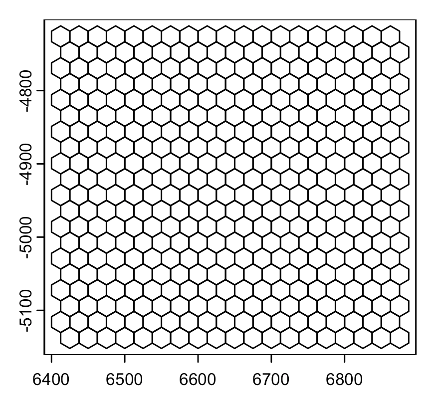
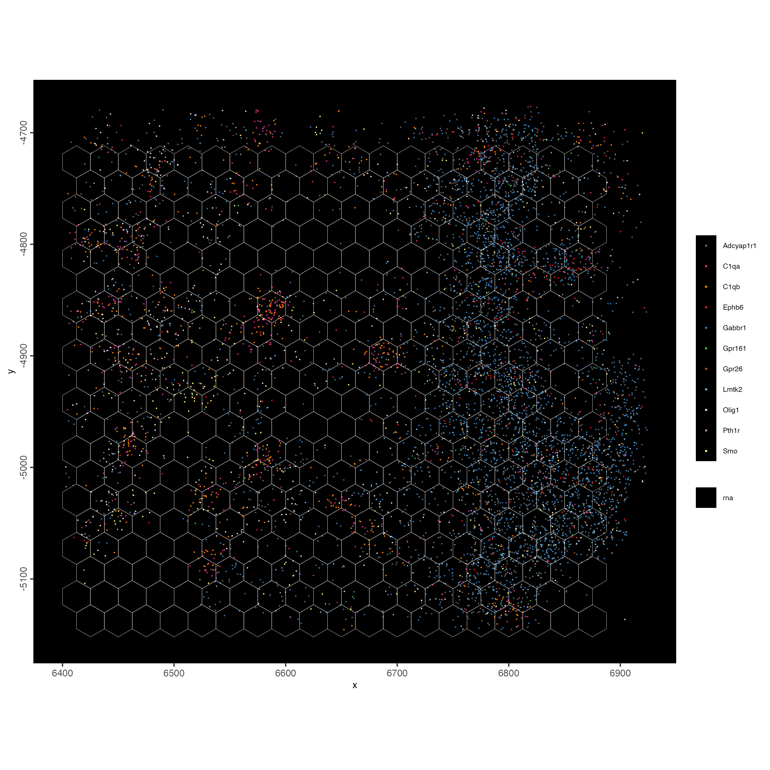
Subcellular data is organized in a grid format. We can aggregate the data into larger bins to reduce the resolution of the data. Giotto Suite can work with any type of polygon information and already provides ready-to-use options for binning data with squares, triangles, and hexagons. Here we will use a hexagon tesselation to aggregate the data into arbitrary bins.
1 Setup Giotto
# Ensure Giotto Suite is installed
if(!"Giotto" %in% installed.packages()) {
  pak::pkg_install("drieslab/Giotto")
}

# Ensure Giotto Data is installed
if(!"GiottoData" %in% installed.packages()) {
  pak::pkg_install("drieslab/GiottoData")
}

library(Giotto)

# Ensure the Python environment for Giotto has been installed
genv_exists <- checkGiottoEnvironment()

if(!genv_exists){
  # The following command need only be run once to install the Giotto environment
  installGiottoEnvironment()
}
2 Get giotto points
The giottoPoints object represents the spatial expression information for each transcript: - gene id - count or UMI - spatial pixel location (x, y)
giotto_points <- GiottoData::loadSubObjectMini("giottoPoints")3 Create giotto polygons
 # create giotto polygons, here we create hexagons
hexbin25 <- tessellate(extent = ext(giotto_points),
                        shape = "hexagon",
                        shape_size = 25,
                        name = "hex100")

plot(hexbin25)
4 Combine Giotto points and polygons to create Giotto object
results_folder <- "/path/to/results/"

python_path <- NULL

instructions <- createGiottoInstructions(save_dir = results_folder,
                                         save_plot = TRUE,
                                         show_plot = FALSE,
                                         return_plot = FALSE,
                                         python_path = python_path)

# gpoints provides spatial gene expression information
# gpolygons provides spatial unit information (here = hexagon tiles)
g <- createGiottoObjectSubcellular(gpoints = list("rna" = giotto_points),
                                   gpolygons = list("hex25" = hexbin25),
                                   instructions = instructions)

# create spatial centroids for each spatial unit (hexagon)
g <- addSpatialCentroidLocations(gobject = g,
                                 poly_info = "hex25")
5 Show the giotto points (transcripts) and polygons (hexagons) together
feature_data <- fDataDT(g)

spatInSituPlotPoints(g,
                     show_image = FALSE,
                     feats = list("rna" = feature_data$feat_ID[10:20]),
                     show_legend = TRUE,
                     spat_unit = "hex25",
                     point_size = 0.25,
                     show_polygon = TRUE,
                     use_overlap = FALSE,
                     polygon_feat_type = "hex25",
                     polygon_bg_color = NA,
                     polygon_color = 'white',
                     polygon_line_size = 0.1,
                     expand_counts = FALSE,
                     jitter = c(25,25))
6 Session info
R version 4.4.2 (2024-10-31)
Platform: x86_64-apple-darwin20
Running under: macOS Sequoia 15.0.1

Matrix products: default
BLAS:   /System/Library/Frameworks/Accelerate.framework/Versions/A/Frameworks/vecLib.framework/Versions/A/libBLAS.dylib
LAPACK: /Library/Frameworks/R.framework/Versions/4.4-x86_64/Resources/lib/libRlapack.dylib;  LAPACK version 3.12.0

locale:
[1] en_US.UTF-8/en_US.UTF-8/en_US.UTF-8/C/en_US.UTF-8/en_US.UTF-8

time zone: America/New_York
tzcode source: internal

attached base packages:
[1] stats     graphics  grDevices utils     datasets  methods   base

other attached packages:
[1] Giotto_4.1.4      GiottoClass_0.4.3

loaded via a namespace (and not attached):
 [1] tidyselect_1.2.1            viridisLite_0.4.2
 [3] farver_2.1.2                dplyr_1.1.4
 [5] GiottoVisuals_0.2.7         fastmap_1.2.0
 [7] SingleCellExperiment_1.26.0 lazyeval_0.2.2
 [9] digest_0.6.37               lifecycle_1.0.4
[11] terra_1.7-78                magrittr_2.0.3
[13] compiler_4.4.2              rlang_1.1.4
[15] tools_4.4.2                 igraph_2.0.3
[17] utf8_1.2.4                  yaml_2.3.10
[19] data.table_1.16.0           knitr_1.48
[21] labeling_0.4.3              S4Arrays_1.4.1
[23] htmlwidgets_1.6.4           reticulate_1.39.0
[25] DelayedArray_0.30.1         RColorBrewer_1.1-3
[27] abind_1.4-8                 withr_3.0.1
[29] purrr_1.0.2                 BiocGenerics_0.50.0
[31] grid_4.4.2                  stats4_4.4.2
[33] fansi_1.0.6                 colorspace_2.1-1
[35] ggplot2_3.5.1               scales_1.3.0
[37] gtools_3.9.5                SummarizedExperiment_1.34.0
[39] cli_3.6.3                   rmarkdown_2.28
[41] crayon_1.5.3                ragg_1.3.3
[43] generics_0.1.3              rstudioapi_0.16.0
[45] httr_1.4.7                  rjson_0.2.23
[47] zlibbioc_1.50.0             parallel_4.4.2
[49] XVector_0.44.0              matrixStats_1.4.1
[51] vctrs_0.6.5                 Matrix_1.7-1
[53] jsonlite_1.8.9              GiottoData_0.2.15
[55] IRanges_2.38.1              S4Vectors_0.42.1
[57] ggrepel_0.9.6               scattermore_1.2
[59] systemfonts_1.1.0           magick_2.8.5
[61] GiottoUtils_0.2.0           plotly_4.10.4
[63] tidyr_1.3.1                 glue_1.8.0
[65] codetools_0.2-20            cowplot_1.1.3
[67] gtable_0.3.5                GenomeInfoDb_1.40.1
[69] GenomicRanges_1.56.1        UCSC.utils_1.0.0
[71] munsell_0.5.1               tibble_3.2.1
[73] pillar_1.9.0                htmltools_0.5.8.1
[75] GenomeInfoDbData_1.2.12     R6_2.5.1
[77] textshaping_0.4.0           evaluate_1.0.0
[79] lattice_0.22-6              Biobase_2.64.0
[81] png_0.1-8                   backports_1.5.0
[83] SpatialExperiment_1.14.0    Rcpp_1.0.13
[85] SparseArray_1.4.8           checkmate_2.3.2
[87] colorRamp2_0.1.0            xfun_0.47
[89] MatrixGenerics_1.16.0       pkgconfig_2.0.3