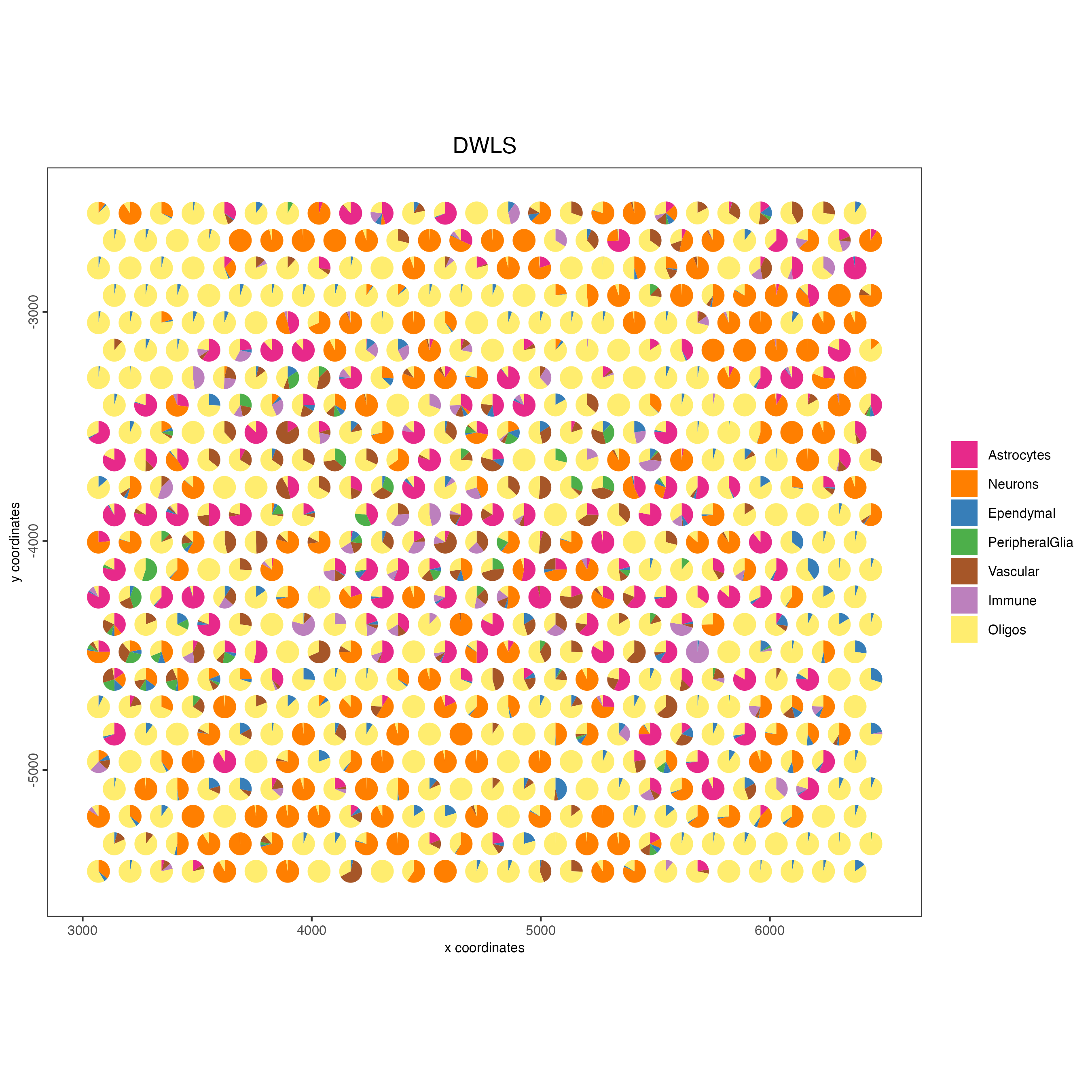
Visium spatial transcriptomics does not provide single-cell resolution, making cell type annotation a harder problem. Giotto provides ways to calculate enrichment of specific cell-type signature gene lists.
Spatial Dampened Weighted Least Squares (DWLS) estimates the proportions of different cell types across spots in a tissue.
1 Setup and load example dataset
# Ensure Giotto Suite is installed
if(!"Giotto" %in% installed.packages()) {
  pak::pkg_install("drieslab/Giotto")
}

# Ensure Giotto Data is installed
if(!"GiottoData" %in% installed.packages()) {
  pak::pkg_install("drieslab/GiottoData")
}

library(Giotto)

# Ensure the Python environment for Giotto has been installed
genv_exists <- checkGiottoEnvironment()

if(!genv_exists){
  # The following command need only be run once to install the Giotto environment
  installGiottoEnvironment()
}
# load the object
g <- GiottoData::loadGiottoMini("visium")
2 Download the single-cell dataset
GiottoData::getSpatialDataset(dataset = "scRNA_mouse_brain",
                              directory = "data/scRNA_mouse_brain")
3 Create the single-cell object and run the normalization step
results_folder <- "path/to/results"

python_path <- NULL

instructions <- createGiottoInstructions(
    save_dir = results_folder,
    save_plot = TRUE,
    show_plot = FALSE,
    python_path = python_path
)

sc_expression <- "data/scRNA_mouse_brain/brain_sc_expression_matrix.txt.gz"
sc_metadata <- data.table::fread("data/scRNA_mouse_brain/brain_sc_metadata.csv")

giotto_SC <- createGiottoObject(expression = sc_expression,
                                instructions = instructions)

giotto_SC <- addCellMetadata(giotto_SC,
                             new_metadata = sc_metadata[,2:129])

giotto_SC <- normalizeGiotto(giotto_SC)
4 Calculate the cell type markers
markers_scran <- findMarkers_one_vs_all(gobject = giotto_SC,
                                        method = "scran",
                                        expression_values = "normalized",
                                        cluster_column = "Class",
                                        min_feats = 3)

top_markers <- markers_scran[, head(.SD, 10), by = "cluster"]$feats
5 Create the signature matrix
sign_matrix <- makeSignMatrixDWLSfromMatrix(
    matrix = getExpression(giotto_SC,
                           values = "normalized",
                           output = "matrix"),
    cell_type = pDataDT(giotto_SC)$Class,
    sign_gene = top_markers)
6 Run the DWLS Deconvolution
This step may take a couple of minutes to run.
g <- runDWLSDeconv(g,
    sign_matrix = sign_matrix
)
7 Visualize
Plot the DWLS deconvolution result creating with pie plots showing the proportion of each cell type per spot.
spatDeconvPlot(g,
    show_image = FALSE,
    radius = 50
)
8 Session info
R version 4.4.2 (2024-10-31)
Platform: x86_64-apple-darwin20
Running under: macOS Sequoia 15.0.1

Matrix products: default
BLAS:   /System/Library/Frameworks/Accelerate.framework/Versions/A/Frameworks/vecLib.framework/Versions/A/libBLAS.dylib
LAPACK: /Library/Frameworks/R.framework/Versions/4.4-x86_64/Resources/lib/libRlapack.dylib;  LAPACK version 3.12.0

locale:
[1] en_US.UTF-8/en_US.UTF-8/en_US.UTF-8/C/en_US.UTF-8/en_US.UTF-8

time zone: America/New_York
tzcode source: internal

attached base packages:
[1] stats     graphics  grDevices utils     datasets  methods   base

other attached packages:
[1] Giotto_4.1.4      GiottoClass_0.4.3

loaded via a namespace (and not attached):
  [1] colorRamp2_0.1.0            rlang_1.1.4
  [3] magrittr_2.0.3              GiottoUtils_0.2.0
  [5] matrixStats_1.4.1           compiler_4.4.2
  [7] DelayedMatrixStats_1.26.0   systemfonts_1.1.0
  [9] png_0.1-8                   vctrs_0.6.5
 [11] RcppZiggurat_0.1.6          quadprog_1.5-8
 [13] pkgconfig_2.0.3             SpatialExperiment_1.14.0
 [15] crayon_1.5.3                fastmap_1.2.0
 [17] backports_1.5.0             magick_2.8.5
 [19] XVector_0.44.0              labeling_0.4.3
 [21] scuttle_1.14.0              utf8_1.2.4
 [23] rmarkdown_2.28              UCSC.utils_1.0.0
 [25] ragg_1.3.3                  purrr_1.0.2
 [27] Rfast_2.1.0                 xfun_0.47
 [29] bluster_1.14.0              zlibbioc_1.50.0
 [31] beachmat_2.20.0             GenomeInfoDb_1.40.1
 [33] jsonlite_1.8.9              DelayedArray_0.30.1
 [35] tweenr_2.0.3                BiocParallel_1.38.0
 [37] terra_1.7-78                irlba_2.3.5.1
 [39] parallel_4.4.2              cluster_2.1.6
 [41] R6_2.5.1                    RColorBrewer_1.1-3
 [43] limma_3.60.4                reticulate_1.39.0
 [45] GenomicRanges_1.56.1        scattermore_1.2
 [47] Rcpp_1.0.13                 SummarizedExperiment_1.34.0
 [49] knitr_1.48                  R.utils_2.12.3
 [51] IRanges_2.38.1              Matrix_1.7-1
 [53] igraph_2.0.3                tidyselect_1.2.1
 [55] rstudioapi_0.16.0           abind_1.4-8
 [57] yaml_2.3.10                 codetools_0.2-20
 [59] lattice_0.22-6              tibble_3.2.1
 [61] Biobase_2.64.0              withr_3.0.1
 [63] evaluate_1.0.0              polyclip_1.10-7
 [65] scatterpie_0.2.4            RcppParallel_5.1.9
 [67] pillar_1.9.0                MatrixGenerics_1.16.0
 [69] checkmate_2.3.2             stats4_4.4.2
 [71] ggfun_0.1.6                 plotly_4.10.4
 [73] generics_0.1.3              S4Vectors_0.42.1
 [75] ggplot2_3.5.1               sparseMatrixStats_1.16.0
 [77] munsell_0.5.1               scales_1.3.0
 [79] GiottoData_0.2.15           gtools_3.9.5
 [81] glue_1.8.0                  metapod_1.12.0
 [83] lazyeval_0.2.2              tools_4.4.2
 [85] GiottoVisuals_0.2.7         BiocNeighbors_1.22.0
 [87] data.table_1.16.0           ScaledMatrix_1.12.0
 [89] locfit_1.5-9.10             fs_1.6.4
 [91] scran_1.32.0                cowplot_1.1.3
 [93] grid_4.4.2                  tidyr_1.3.1
 [95] edgeR_4.2.1                 colorspace_2.1-1
 [97] SingleCellExperiment_1.26.0 GenomeInfoDbData_1.2.12
 [99] ggforce_0.4.2               BiocSingular_1.20.0
[101] cli_3.6.3                   rsvd_1.0.5
[103] textshaping_0.4.0           fansi_1.0.6
[105] S4Arrays_1.4.1              viridisLite_0.4.2
[107] dplyr_1.1.4                 gtable_0.3.5
[109] yulab.utils_0.1.7           R.methodsS3_1.8.2
[111] digest_0.6.37               progressr_0.14.0
[113] BiocGenerics_0.50.0         SparseArray_1.4.8
[115] ggrepel_0.9.6               dqrng_0.4.1
[117] farver_2.1.2                rjson_0.2.23
[119] htmlwidgets_1.6.4           htmltools_0.5.8.1
[121] R.oo_1.26.0                 lifecycle_1.0.4
[123] httr_1.4.7                  statmod_1.5.0
[125] MASS_7.3-61