Multi-omics Mouse Embryo DBiT-Seq
Source:vignettes/mouse_embryo_dbitseq.Rmd
mouse_embryo_dbitseq.Rmd1 Dataset explanation
The dataset was created by Liu, et al 2020 and downloaded from https://www.ncbi.nlm.nih.gov/geo/query/acc.cgi?acc=GSE137986. For running this tutorial, we will use the dataset E10 Whole (50 μm) 2.
For running this tutorial, we need to download the RNA expression matrix (GSE137986_RAW/GSM4189613_0702cL.tsv.gz) and the Protein counts matrix (GSE137986_RAW/GSM4202307_0702aL.tsv.gz), while the spatial coordinates will be taken from the cell_ids.
2 Start Giotto
Make sure you have the Giotto package and environment installed. If you have installation problems, visit the Installation guidelines and FAQ section.
# Ensure Giotto Suite is installed
if(!"Giotto" %in% installed.packages()) {
  pak::pkg_install("drieslab/Giotto")
}

# Ensure the Python environment for Giotto has been installed
genv_exists <- Giotto::checkGiottoEnvironment()
if(!genv_exists){
  # The following command need only be run once to install the Giotto environment
  Giotto::installGiottoEnvironment()
}
3 Read the data
Read the RNA and Protein count matrices. You expect to have and RNA expression matrix with 22846 genes and 901 cells, and a Protein matrix with 22 proteins and 901 cells.
library(Giotto)

data_path <- "/path/to/data/"

## RNA
rna_expression <- read.table(paste0(data_path, "GSE137986_RAW/GSM4189613_0702cL.tsv.gz"),
                            sep = "\t",
                            header = TRUE)
rownames(rna_expression) <- rna_expression$X
## Protein
protein_expression <- read.table(paste0(data_path, "GSE137986_RAW/GSM4202307_0702aL.tsv.gz"),
                                sep = "\t",
                                header = TRUE)
rownames(protein_expression) <- protein_expression$X
Transpose the matrices. DBiT-seq provides the counts matrices in a cell x gene format, but we need a gene x cell matrix for creating the Giotto object.
Extract the spatial coordinates. This dataset did not provide a separated spatial coordinates file, but we can get the spatial information from the cell ids.
spatial_coords <- data.frame(cell_ID = colnames(rna_expression))
spatial_coords <- cbind(spatial_coords,
                       tidyr::separate(spatial_coords, cell_ID, c("x","y"), sep = "x"))

spatial_coords$x <- as.numeric(spatial_coords$x)
spatial_coords$y <- as.numeric(spatial_coords$y)*-1
4 Create the Giotto object
Use the Giotto instructions to set the behavior of the Giotto object, such as whether you prefer to save the generated plots or only visualize them. This instructions will become the default for future plotting functions, but you can also use the functions arguments to change the saving options.
results_folder <- "/path/to/results/"

instructions <- createGiottoInstructions(results_folder = results_folder,
                                         save_plot = TRUE,
                                         show_plot = FALSE,
                                         return_plot = FALSE)

giottoObject <- createGiottoObject(expression = list(raw = rna_expression,
                                                     raw = protein_expression),
                                   expression_feat = c("rna", "protein"),
                                   spatial_locs = spatial_coords,
                                   instructions = instructions)
5 Processing
5.1 Filtering
We need to remove those spots that contain a very small number of features (genes or proteins), as well as features that are not expressed in enough spots across the sample.
Use the argument min_det_feats_per_cell to set the minimal number of features (genes or proteins) expected per spot. Those spots with less genes or proteins than the provided number will be removed.
Use the argument feat_det_in_min_cells to set the minimal number of spots where each gene or protein should be expressed to be considered in the dataset. Those genes or proteins expressed in less spots than the provided number will be removed.
## RNA
giottoObject <- filterGiotto(gobject = giottoObject,
                             expression_threshold = 1,
                             feat_det_in_min_cells = 1,
                             min_det_feats_per_cell = 1,
                             expression_values = "raw",
                             verbose = TRUE)

## Protein
giottoObject <- filterGiotto(gobject = giottoObject,
                             spat_unit = "cell",
                             feat_type = "protein",
                             expression_threshold = 1,
                             feat_det_in_min_cells = 1,
                             min_det_feats_per_cell = 1,
                             expression_values = "raw",
                             verbose = TRUE)
5.2 Normalization
Normalize the gene or protein counts by cell, then use the argument scalefactor to set the scale factor to use after library size normalization. The default value is 6000, but you can use a different one.
## RNA
giottoObject <- normalizeGiotto(gobject = giottoObject,
                                scalefactor = 6000,
                                verbose = TRUE)

## Protein
giottoObject <- normalizeGiotto(gobject = giottoObject,
                                spat_unit = "cell",
                                feat_type = "protein",
                                scalefactor = 6000,
                                verbose = TRUE)
5.3 Statistics
Add cell and feature statistics (optional). These values can be used as Quality control, you usually expect to have enough genes or proteins per spot, but the minimal number depends on the experiment design and technology used.
## RNA
giottoObject <- addStatistics(gobject = giottoObject)
spatPlot2D(giottoObject,
spat_unit = "cell",
feat_type = "rna",
cell_color = "nr_feats",
color_as_factor = FALSE,
point_size = 3.5)
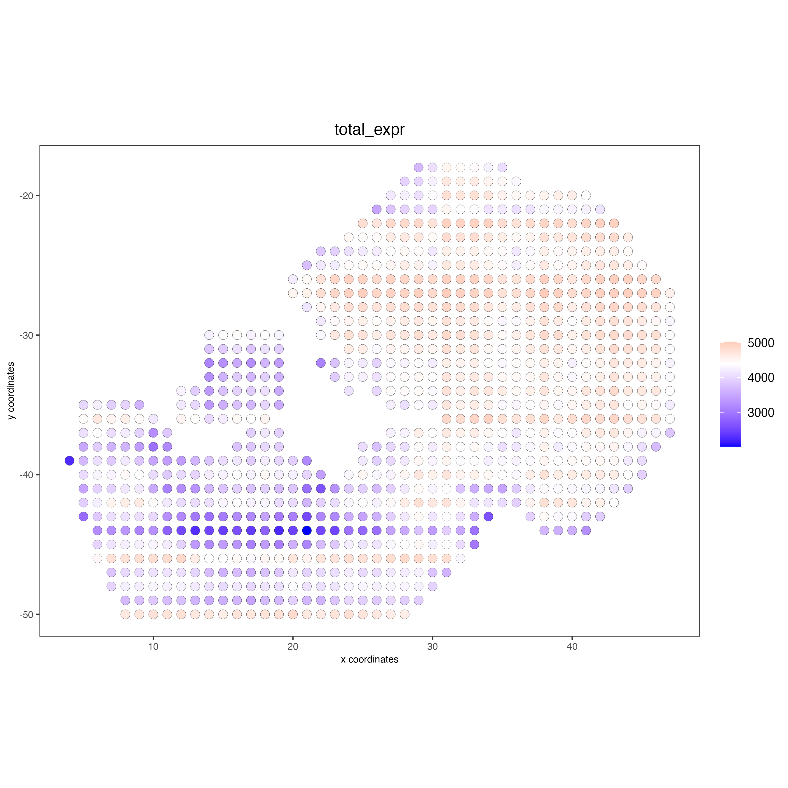
spatPlot2D(giottoObject,
cell_color = "total_expr",
color_as_factor = FALSE,
point_size = 3.5)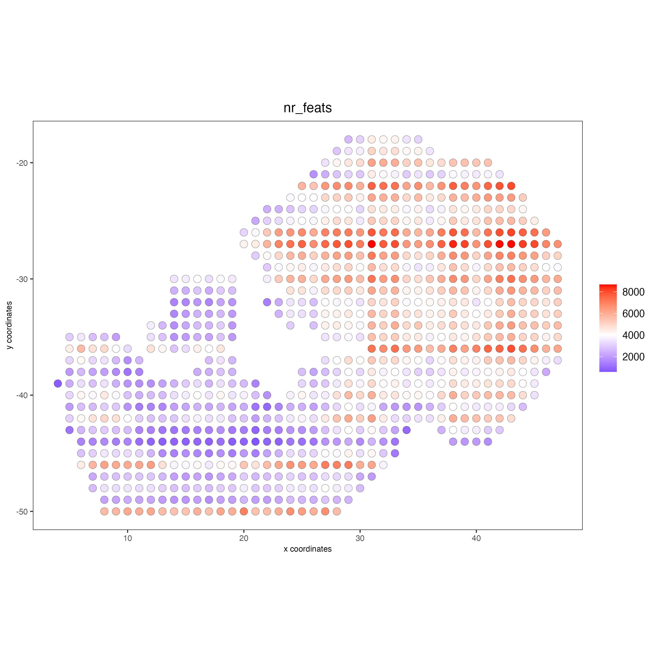
## Protein
giottoObject <- addStatistics(gobject = giottoObject,
                              spat_unit = "cell",
                              feat_type = "protein")

spatPlot2D(giottoObject,
           spat_unit = "cell",
           feat_type = "protein",
           cell_color = "total_expr",
           color_as_factor = FALSE,
           point_size = 3.5)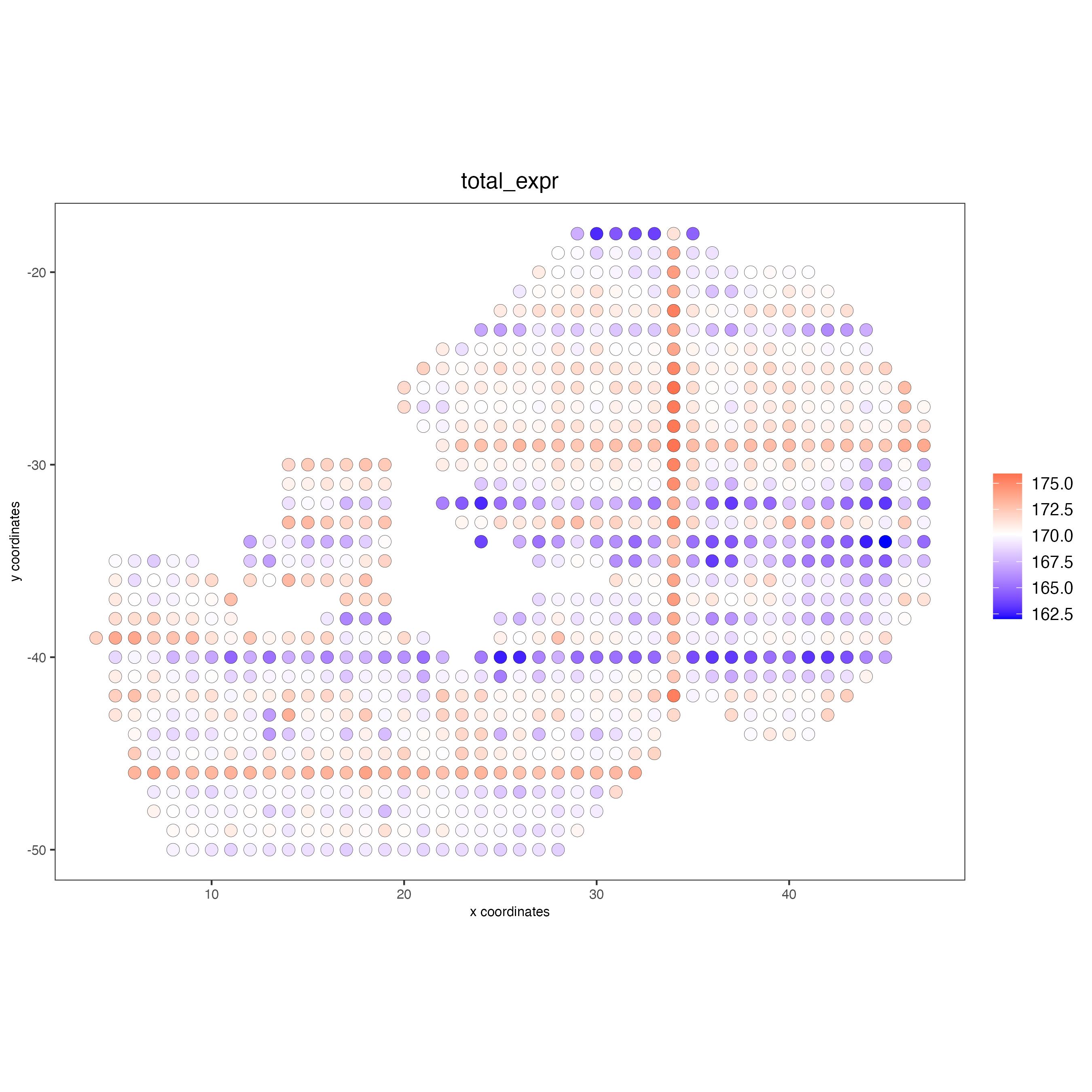
6 Dimension Reduction
6.1 Identify highly variable features (HVF)
When having whole transcriptome RNA information, you may want to identify the genes with highest variability and use them for the Principal Components Analysis. This step is not needed for the Protein modality, since the number of proteins is very limited.
giottoObject <- calculateHVF(gobject = giottoObject)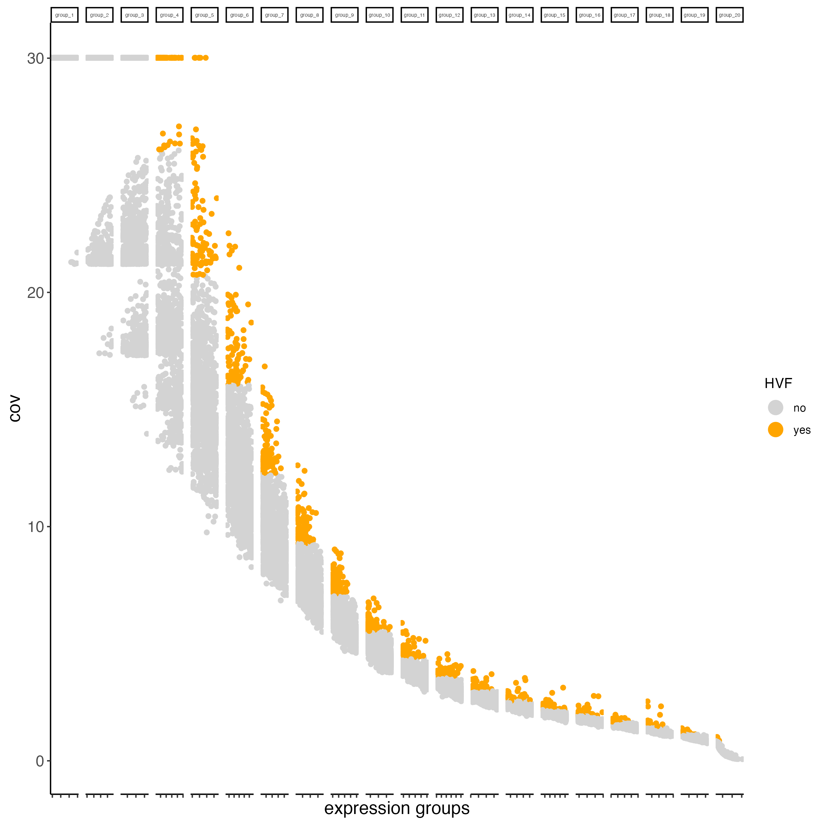
6.2 PCA
The Principal component Analysis will help to reduce the number of dimensions in the dataset. For the RNA modality, we will use the previously calculated HVFs, but for the protein modality we will use all the proteins available in the dataset.
The screeplot will show how much of the variance of your dataset is explain by each Principal Component. Usually this helps to estimate the number of Principal Components that you should consider for downstream steps.
# RNA
giottoObject <- runPCA(gobject = giottoObject)
screePlot(giottoObject,
          ncp = 30)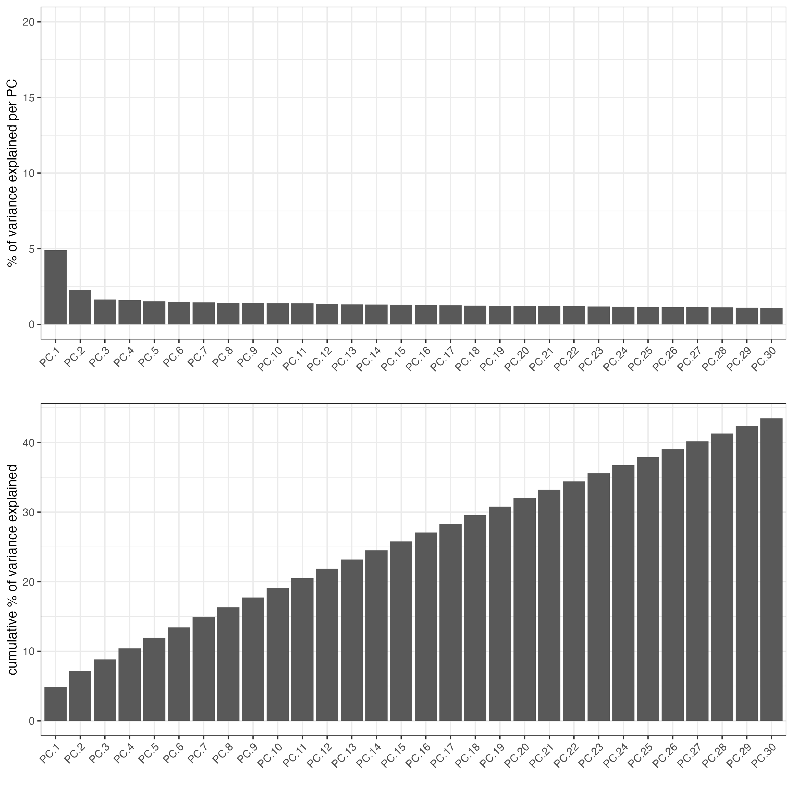
plotPCA(gobject = giottoObject)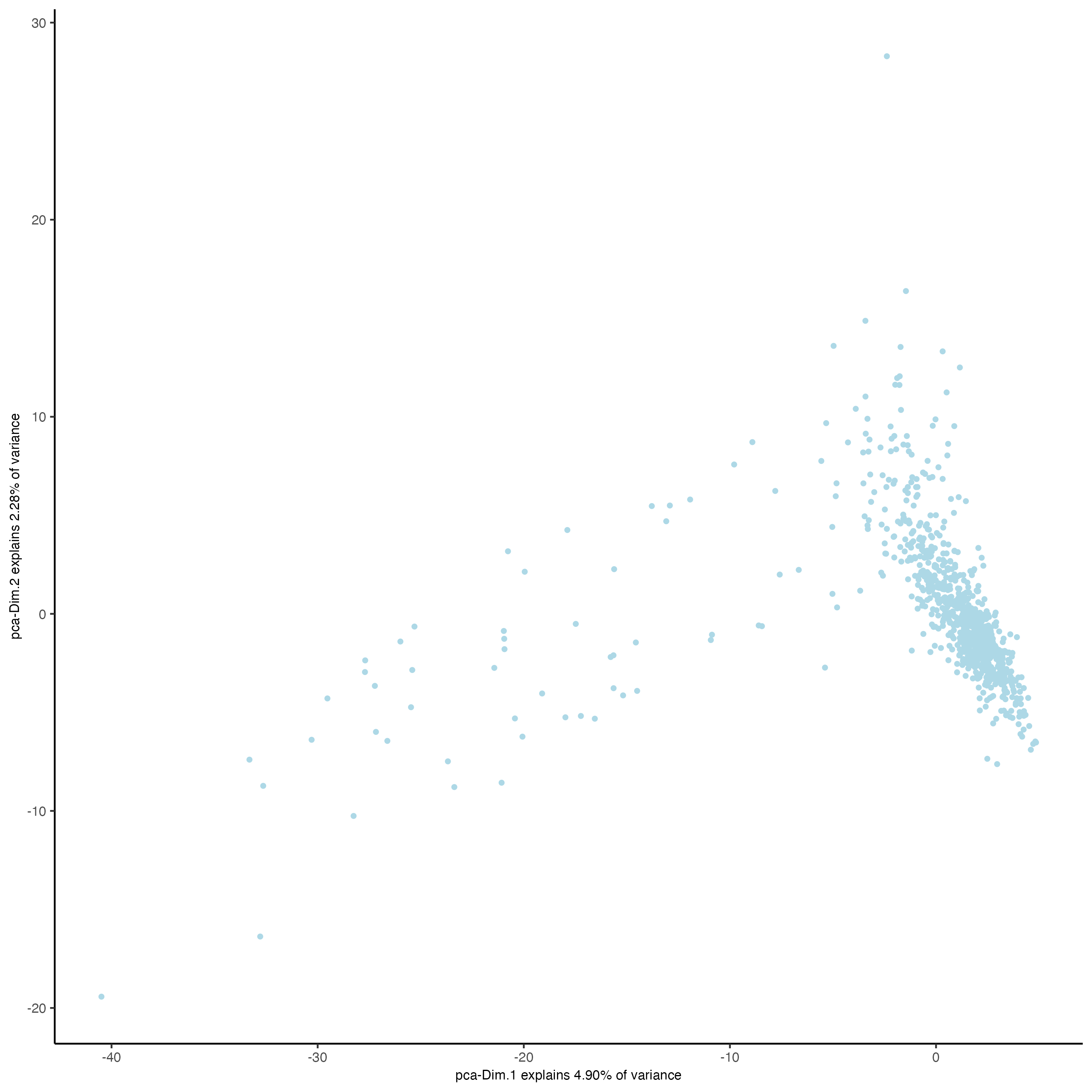
# Protein
giottoObject <- runPCA(gobject = giottoObject,
                       spat_unit = "cell",
                       feat_type = "protein")
screePlot(giottoObject,
          spat_unit = "cell",
          feat_type = "protein",
          ncp = 30)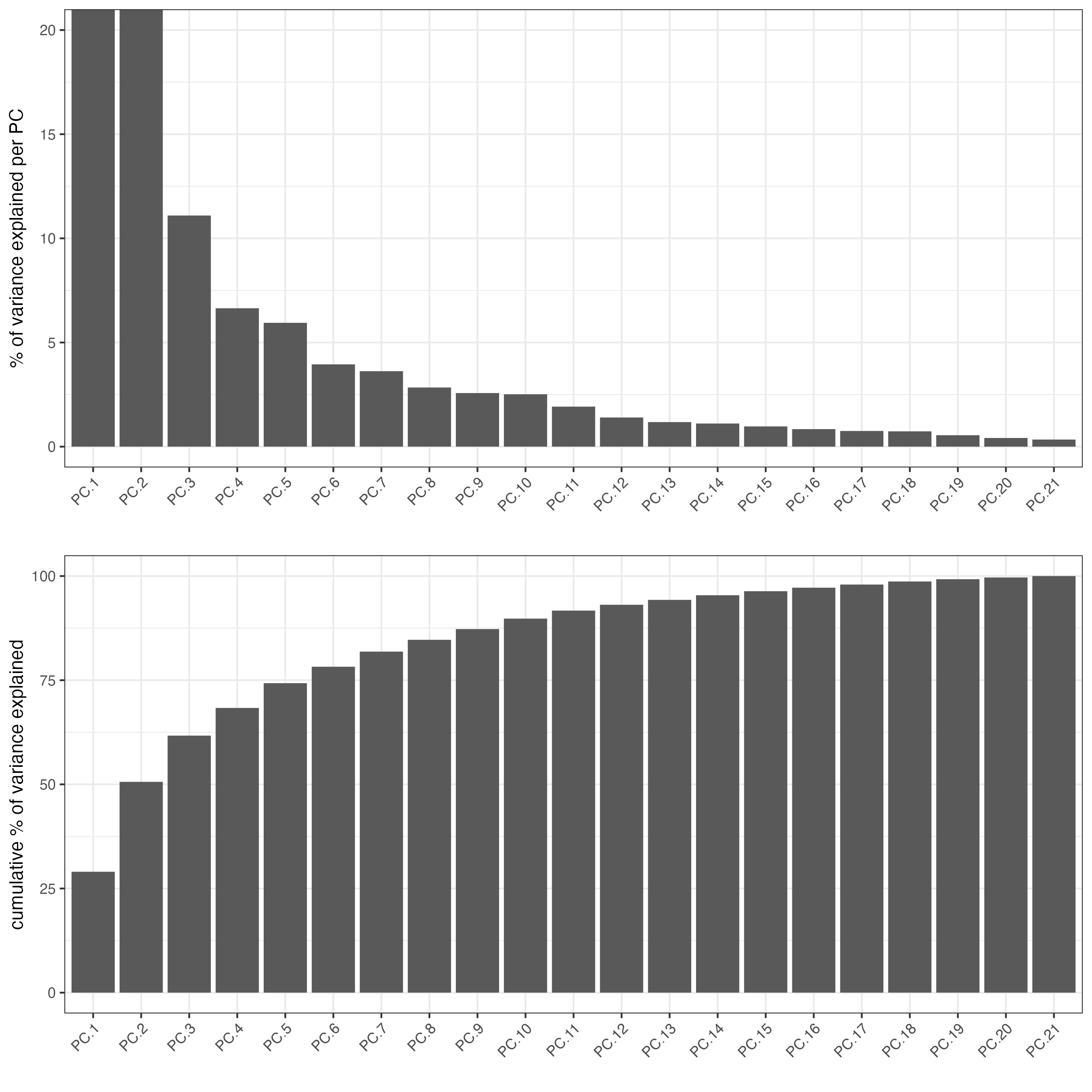
plotPCA(gobject = giottoObject,
        spat_unit = "cell",
        feat_type = "protein")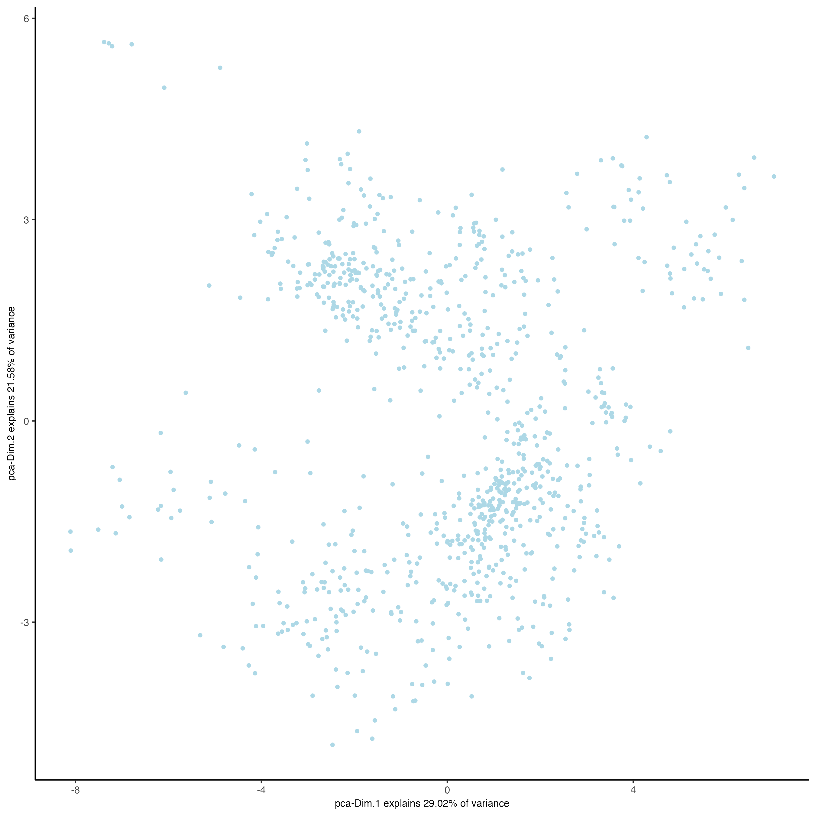
7 Clustering
7.1 UMAP
Unlike PCA, Uniform Manifold Approximation and Projection (UMAP) do not assume linearity. After running the PCA, UMAP allows you to visualize the dataset in 2D.
# RNA
giottoObject <- runUMAP(giottoObject,
                        dimensions_to_use = 1:10)
plotUMAP(gobject = giottoObject)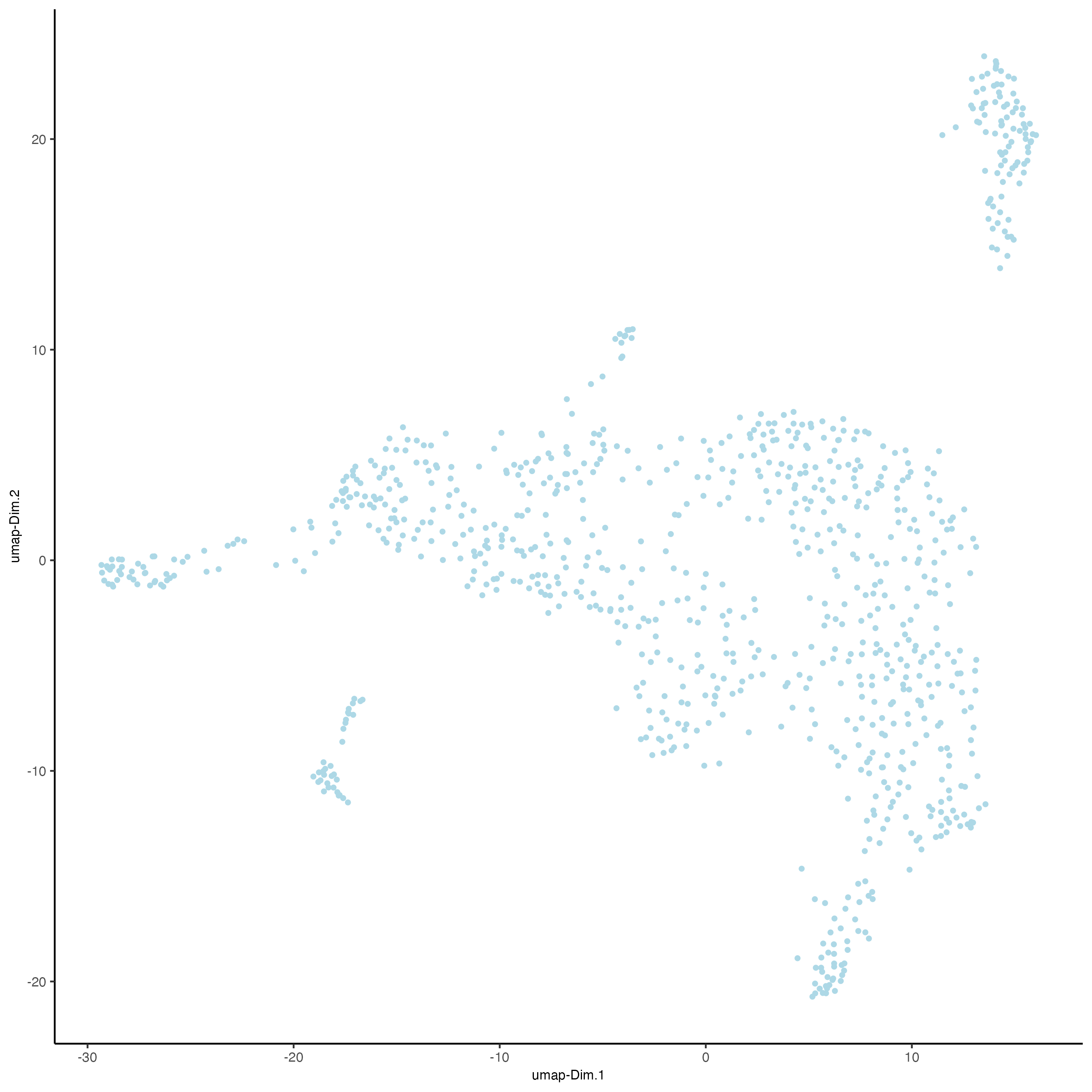
# Protein
giottoObject <- runUMAP(giottoObject,
                        spat_unit = "cell",
                        feat_type = "protein",
                        dimensions_to_use = 1:10)
plotUMAP(gobject = giottoObject,
         spat_unit = "cell",
         feat_type = "protein")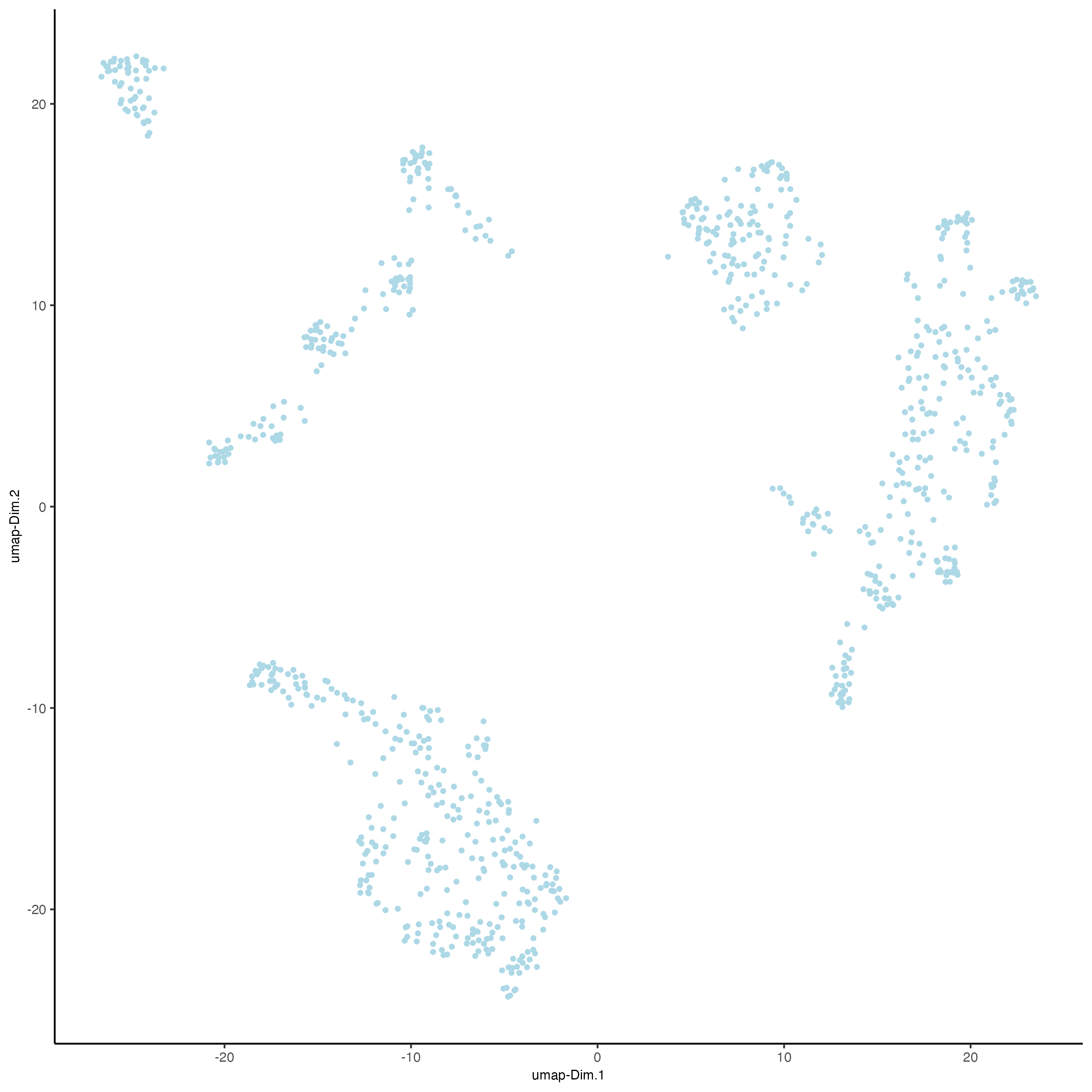
7.2 Create shared nearest network (sNN) and perform Leiden clustering
createNearestNetwork() calculates the nearest neighbors to each spot based on their gene or protein expression. There are two methods available for the calculation, sNN (default) and kNN, You can also use the parameters dimensions_to_use to set how many dimensions from the PCA will be used for the network calculation and how many neighbors (k) to calculate.
Once you have calculated the spots network, we can cluster the spots based on their similarity. By default, doLeidenCluster uses a resolution of 1, but you can change this value, which usually ranges from 0 (lowest resolution) to 1, but can go further if a higher resolution is needed.
# RNA
giottoObject <- createNearestNetwork(gobject = giottoObject,
                                     dimensions_to_use = 1:10,
                                     k = 30)

giottoObject <- doLeidenCluster(gobject = giottoObject,
                                resolution = 1,
                                n_iterations = 1000)

# Protein
giottoObject <- createNearestNetwork(gobject = giottoObject,
                                     spat_unit = "cell",
                                     feat_type = "protein",
                                     dimensions_to_use = 1:10,
                                     k = 30)

giottoObject <- doLeidenCluster(gobject = giottoObject,
                                spat_unit = "cell",
                                feat_type = "protein",
                                resolution = 1,
                                n_iterations = 1000)
7.3 Visualize UMAP cluster results
# RNA
plotUMAP(gobject = giottoObject,
         cell_color = "leiden_clus",
         show_NN_network = FALSE,
         point_size = 2,
         title = "",
         axis_text = 14,
         axis_title = 18,
         legend_text = 14)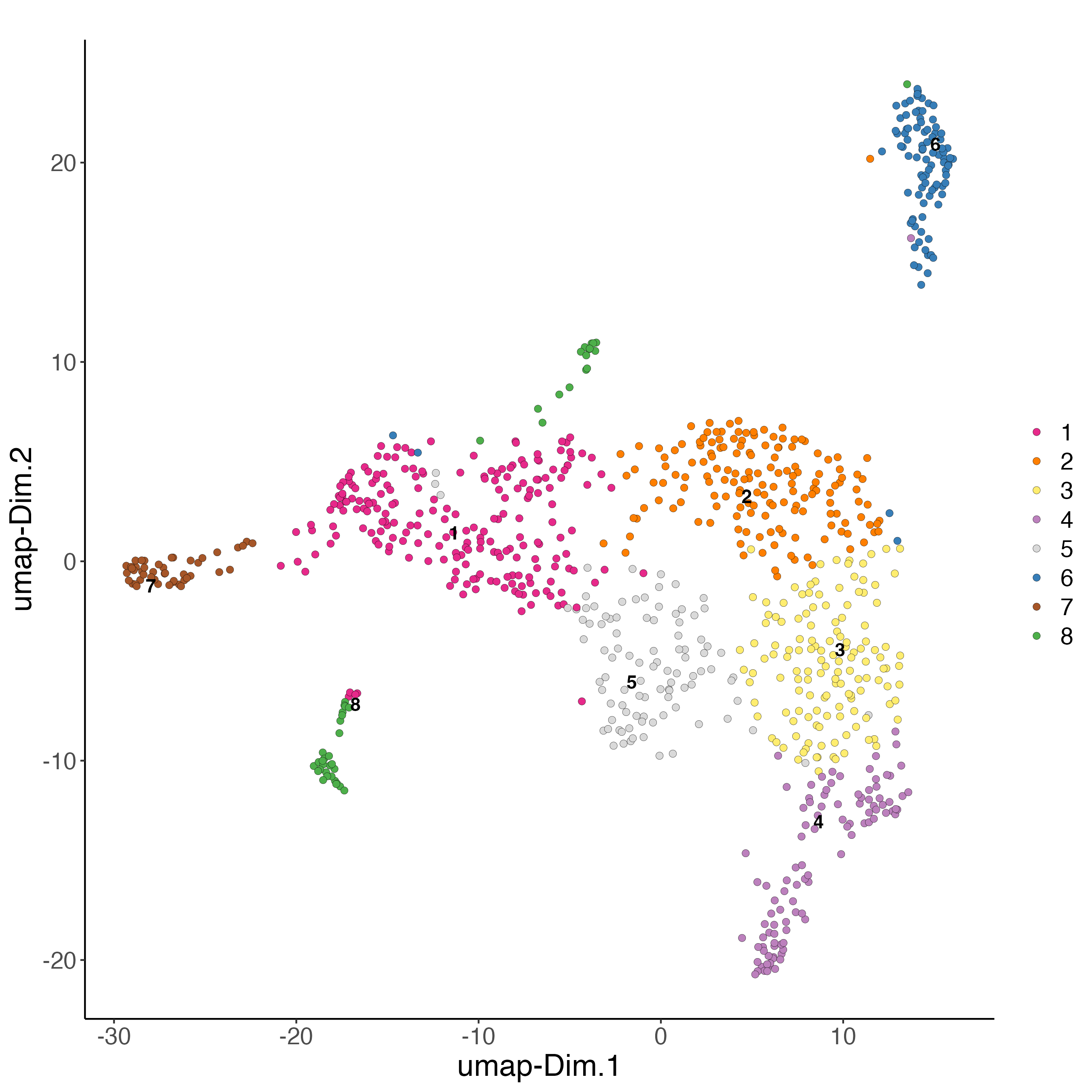
# Protein
plotUMAP(gobject = giottoObject,
         spat_unit = "cell",
         feat_type = "protein",
         cell_color = "leiden_clus",
         show_NN_network = FALSE,
         point_size = 2,
         title = "",
         axis_text = 14,
         axis_title = 18,
         legend_text = 14)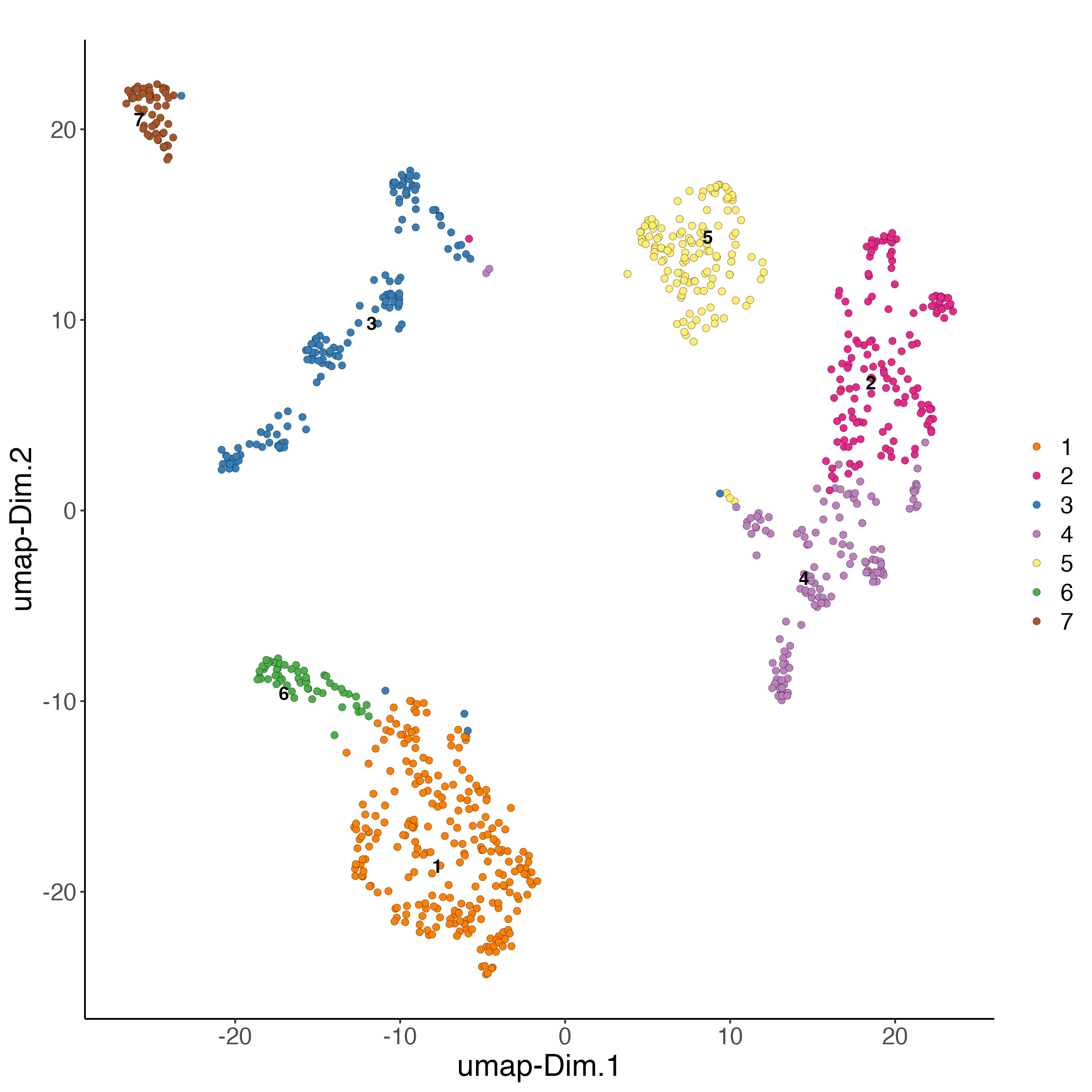
7.4 Visualize spatial results
# RNA
spatPlot2D(gobject = giottoObject,
           show_image = FALSE,
           cell_color = "leiden_clus",
           point_size = 3.5,
           title = "",
           axis_text = 14,
           axis_title = 18,
           legend_text = 14)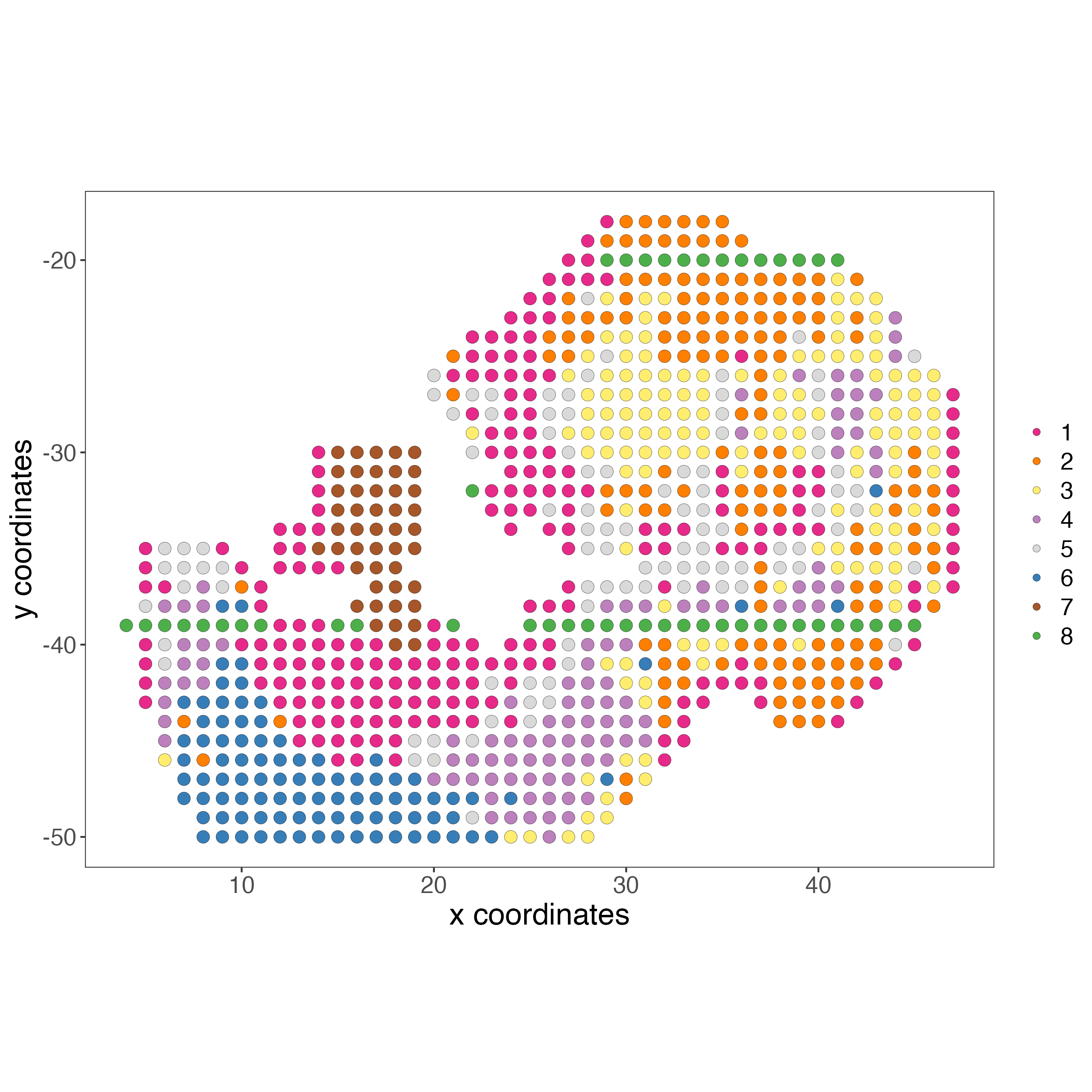
# Protein
spatPlot2D(gobject = giottoObject,
           spat_unit = "cell",
           feat_type = "protein",
           show_image = FALSE,
           cell_color = "leiden_clus",
           point_size = 3.5,
           title = "",
           axis_text = 14,
           axis_title = 18,
           legend_text = 14)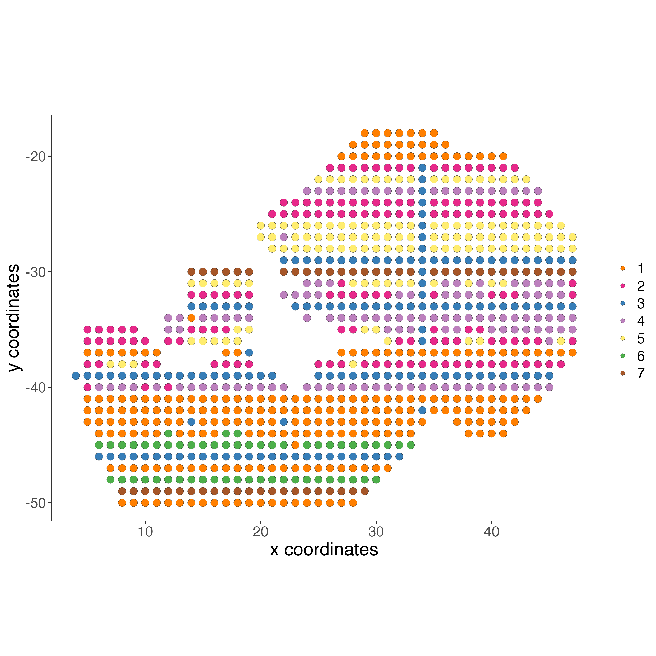
8 Multi-omics integration
The Weighted Nearest Neighbors allows to integrate the modalities acquired from the same sample. WNN will re-calculate the clustering to provide an integrated umap and leiden clustering. For running WNN, the Giotto object must contain the results of running PCA calculation for each modality.
8.1 Calculate kNN
First, we need a nearest network using the kNN method; if you used this method in the clustering step instead of sNN, you can skip this step.
# RNA
giottoObject <- createNearestNetwork(gobject = giottoObject,
                                     type = "kNN",
                                     dimensions_to_use = 1:10,
                                     k = 20)

# Protein
giottoObject <- createNearestNetwork(gobject = giottoObject,
                                     spat_unit = "cell",
                                     feat_type = "protein",
                                     type = "kNN",
                                     dimensions_to_use = 1:10,
                                     k = 20)
8.2 Run WNN
runWNN will calculate the weight of each modality for each spot and will store the result in the Giotto object under the multiomics slot.
giottoObject <- runWNN(giottoObject,
                       spat_unit = "cell",
                       modality_1 = "rna",
                       modality_2 = "protein",
                       pca_name_modality_1 = "pca",
                       pca_name_modality_2 = "protein.pca",
                       k = 20,
                       verbose = TRUE)
8.3 Run Integrated umap
Using the weights matrix from the previous step, an integrated kNN and UMAP will be calculated, which reflects the integration of the two omics.
giottoObject <- runIntegratedUMAP(giottoObject,
                                  modality1 = "rna",
                                  modality2 = "protein",
                                  spread = 7,
                                  min_dist = 1,
                                  force = FALSE)
8.4 Calculate integrated clusters
The final step is calculating the Leiden clusters again, using the integrated information from the previous step. These clusters consider the weight of each modality per spot.
giottoObject <- doLeidenCluster(gobject = giottoObject,
                                spat_unit = "cell",
                                feat_type = "rna",
                                nn_network_to_use = "kNN",
                                network_name = "integrated_kNN",
                                name = "integrated_leiden_clus",
                                resolution = 1)
plotUMAP(gobject = giottoObject,
         spat_unit = "cell",
         feat_type = "rna",
         cell_color = "integrated_leiden_clus",
         dim_reduction_name = "integrated.umap",
         point_size = 2,
         title = "",
         axis_text = 14,
         axis_title = 18,
         legend_text = 14)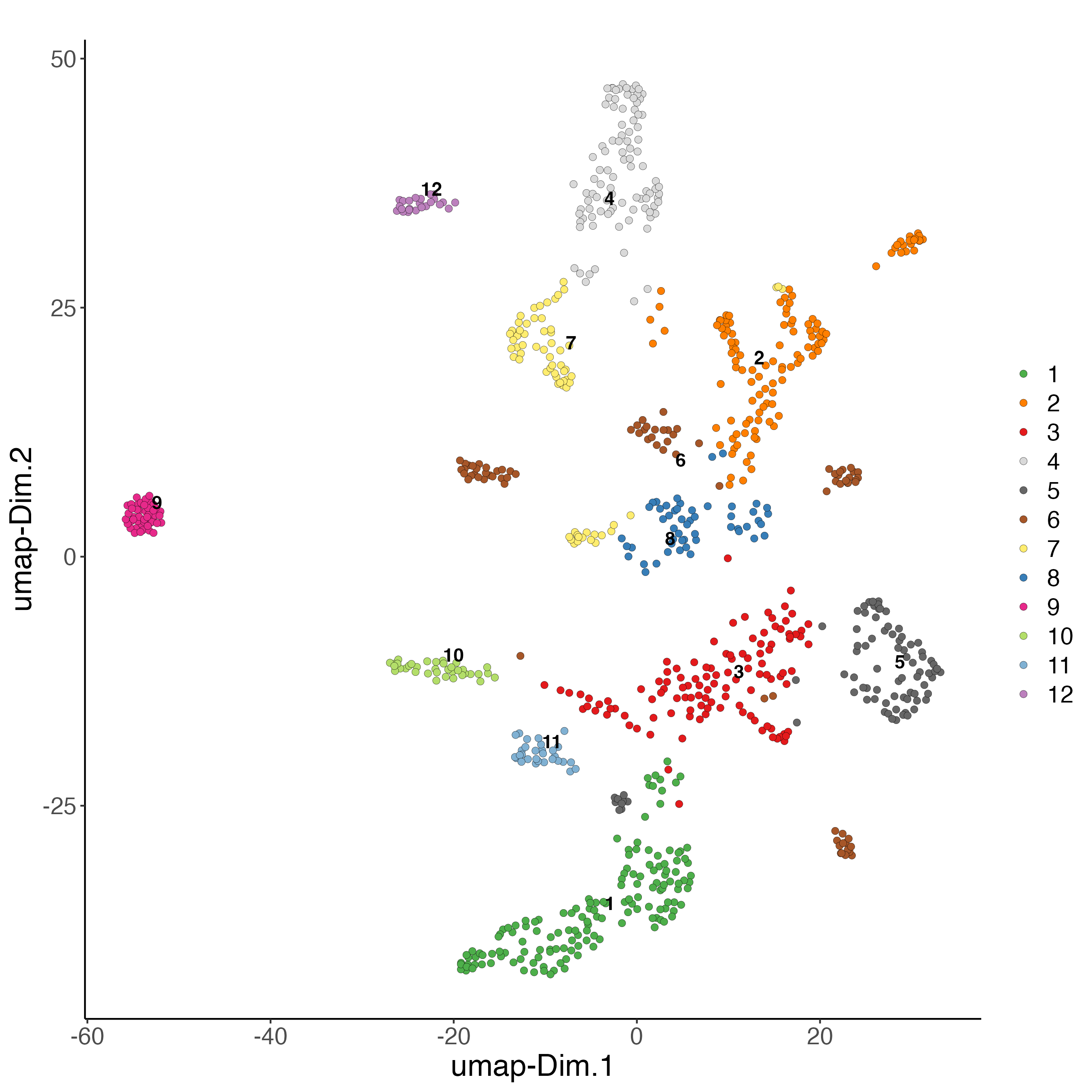
spatPlot2D(giottoObject,
           spat_unit = "cell",
           feat_type = "rna",
           cell_color = "integrated_leiden_clus",
           point_size = 3.5,
           show_image = FALSE,
           title = "",
           axis_text = 14,
           axis_title = 18,
           legend_text = 14)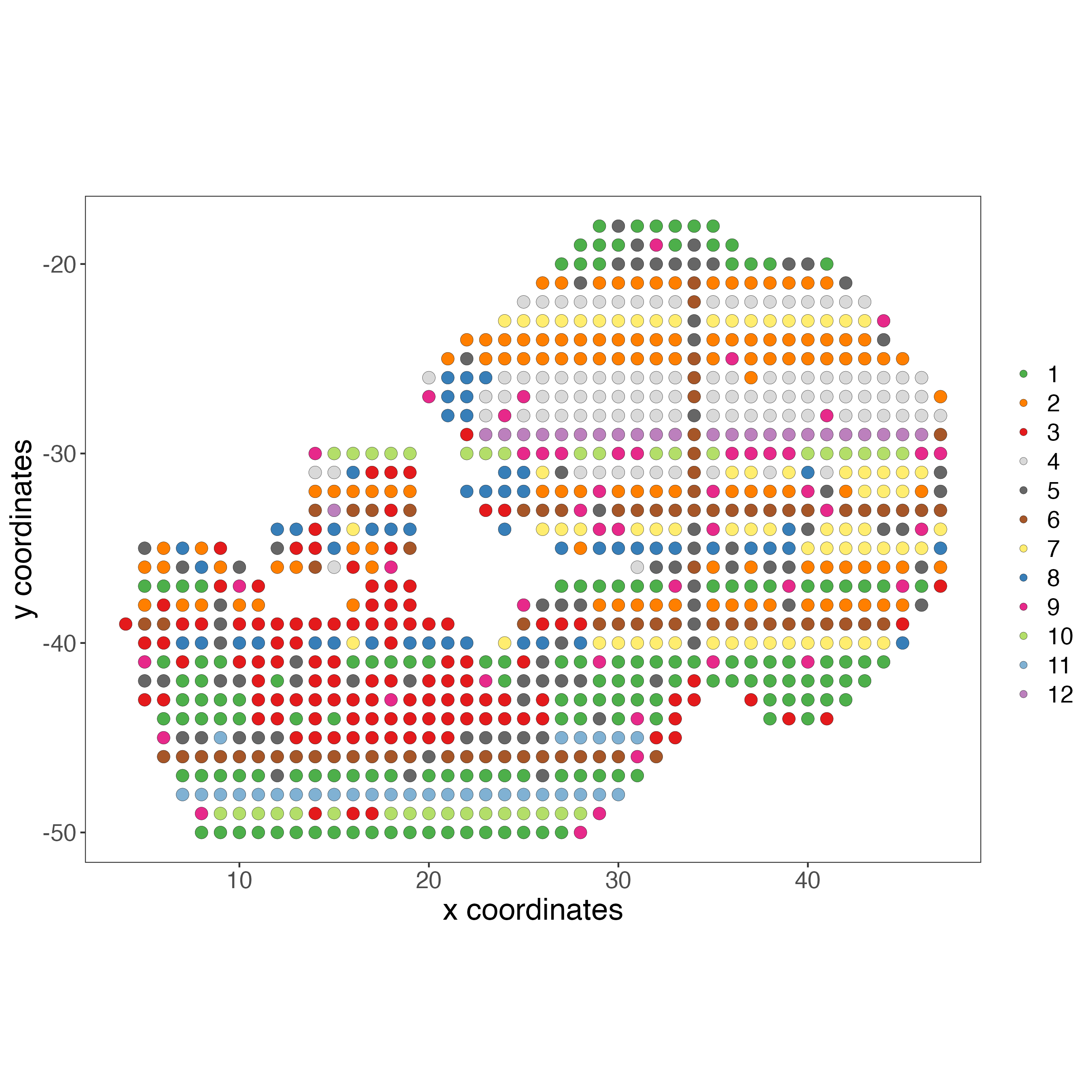
9 Deconvolution
We used the scRNAseq from Cao et al., 2019 as reference. J. Cao, M. Spielmann, X. Qiu, X. Huang, D.M. Ibrahim, A.J. Hill, F. Zhang, S. Mundlos, L. Christiansen, F.J. Steemers, et al. The single-cell transcriptional landscape of mammalian organogenesis. You can download the gene_count_cleaned_sampled_100k.RDS file from here.
9.1 Preparation of the scRNAseq
Read the counts object and the metadata file with cell type annotation.
# read single cell processed object
gene_count_cleaned_sampled_100k <- readRDS(paste0(data_path, "gene_count_cleaned_sampled_100k.RDS"))

# download cell annotations
download.file(url = "https://shendure-web.gs.washington.edu/content/members/cao1025/public/mouse_embryo_atlas/cell_annotate.csv",
              destfile = paste0(data_path, "cell_annotate.csv"))

# or run in your terminal: wget https://shendure-web.gs.washington.edu/content/members/cao1025/public/mouse_embryo_atlas/cell_annotate.csv

cell_annotation <- data.table::fread(paste0(data_path, "cell_annotate.csv"))
cell_annotation <- cell_annotation[, c("sample", "Total_mRNAs", "num_genes_expressed", "Main_cell_type")]
colnames(cell_annotation)[1] <- "cell_ID"

cell_annotation <- cell_annotation[cell_annotation$cell_ID %in% colnames(gene_count_cleaned_sampled_100k),]
Create the single-cell Giotto object and keep only the cells included in the metadata file. Then add the cell type annotation to the metadata of the Giotto object.
sc_giotto <- createGiottoObject(expression = gene_count_cleaned_sampled_100k)

sc_giotto <- subsetGiotto(sc_giotto,
                          cell_ids = cell_annotation$cell_ID)

sc_giotto <- addCellMetadata(sc_giotto,
                             new_metadata = cell_annotation)
For the deconvolution step, we need the normalized counts of the single-cell data. Use normalizeGiotto to perform the normalization step. Here we are setting the scaling options to FALSE because only the normalized counts are needed, but you can change them to TRUE if you prefer to also scale the object.
sc_giotto <- normalizeGiotto(sc_giotto,
                             log_norm = FALSE,
                             scale_feats = FALSE,
                             scale_cells = FALSE)
Use the cell type annotation to find their marker genes based on ther normalized expression. The list of marker genes will be used to create a signature matrix in the next step.
markers_scran <- findMarkers_one_vs_all(gobject = sc_giotto,
                                        method = "scran",
                                        expression_values = "normalized",
                                        cluster_column = "Main_cell_type",
                                        min_feats = 3)

topgenes_scran <- unique(markers_scran[, head(.SD, 30), by = "cluster"][["feats"]])
Create DWLS matrix. The signature matrix takes into account the marker genes per cell type and their normalized expression in the single-cell object.
DWLS_matrix_direct <- makeSignMatrixDWLSfromMatrix(
  matrix = getExpression(sc_giotto,
                         values = "normalized",
                         output = "matrix"),
  cell_type = pDataDT(sc_giotto)$Main_cell_type,
  sign_gene = topgenes_scran)
Fix gene names. This dataset contains some ENSEMBL gene ids, we need to homogenize the ids to match the nomenclature of the RNA matrix in the spatial object.
# download gene annotations
download.file(url = "https://shendure-web.gs.washington.edu/content/members/cao1025/public/mouse_embryo_atlas/gene_annotate.csv",
              destfile = paste0(data_path, "gene_annotate.csv"))

sc_gene_names <- read.csv(paste0(data_path, "gene_annotate.csv"))

ENSMUS_names <- rownames(DWLS_matrix_direct)
sc_gene_names <- sc_gene_names[sc_gene_names$gene_id %in% ENSMUS_names,]

rownames(DWLS_matrix_direct) <- sc_gene_names$gene_short_name
9.2 Run deconvolution
Use the single-cell signature matrix to perform the deconvolution of the spatial object.
# run DWLS using integrated leiden clusters
giottoObject <- runDWLSDeconv(gobject = giottoObject,
                              sign_matrix = DWLS_matrix_direct,
                              cluster_column = "integrated_leiden_clus")
Plot DWLS deconvolution result. The DWLS method will retrieve as output a table with the proportion of each cell type by spot, you can use this information to create a pie plot per spot.
# Plot DWLS deconvolution result with Pie plots dataset 1
spatDeconvPlot(giottoObject,
               show_image = FALSE,
               radius = 0.5,
               return_plot = TRUE,
               save_plot = TRUE,
               save_param = list(save_name = "integrated_deconvolution"),
               title = "",
               axis_text = 14,
               axis_title = 18,
               legend_text = 0,
               background_color = "black")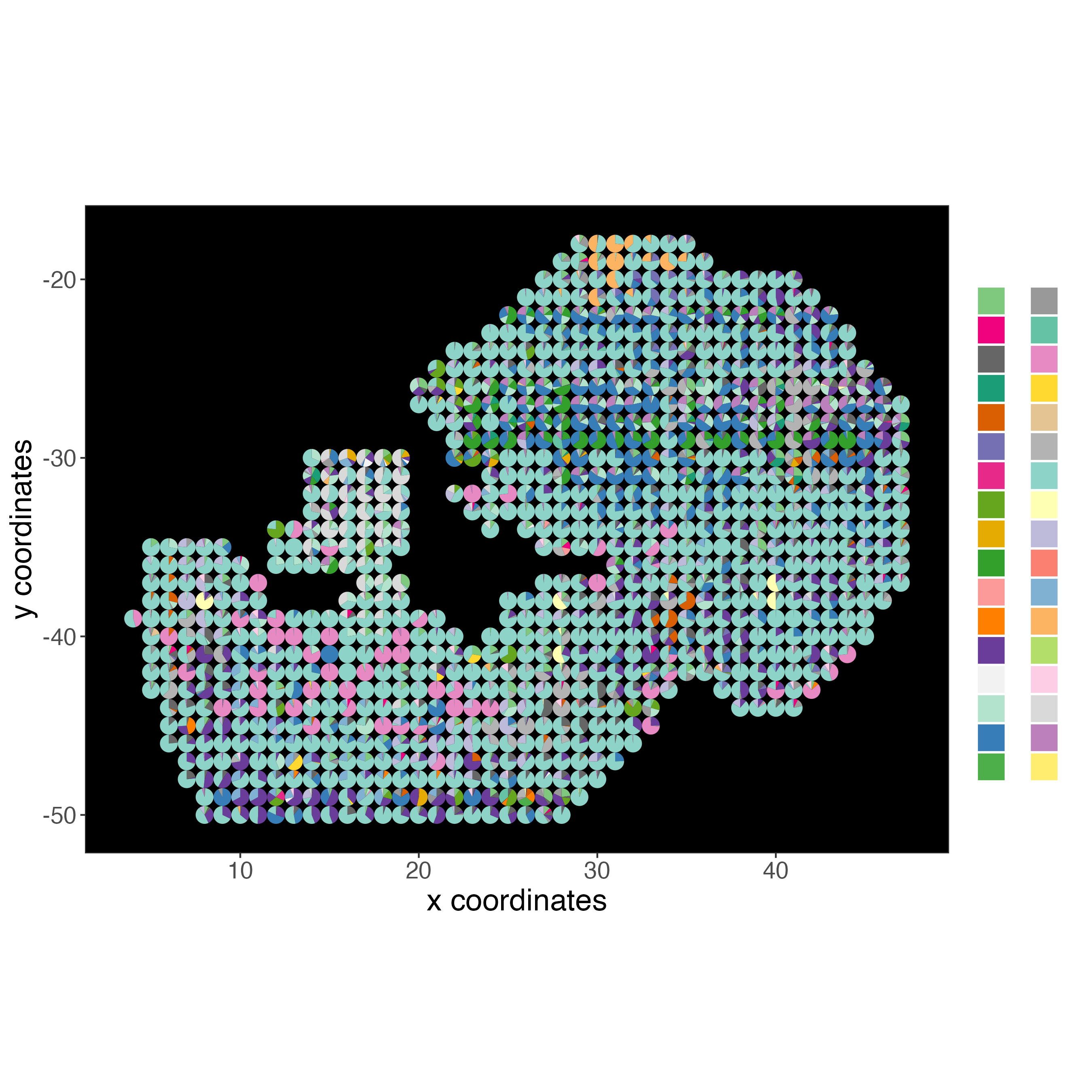
10 Session Info
R version 4.3.2 (2023-10-31)
Platform: x86_64-apple-darwin20 (64-bit)
Running under: macOS Sonoma 14.3.1

Matrix products: default
BLAS:   /System/Library/Frameworks/Accelerate.framework/Versions/A/Frameworks/vecLib.framework/Versions/A/libBLAS.dylib
LAPACK: /Library/Frameworks/R.framework/Versions/4.3-x86_64/Resources/lib/libRlapack.dylib;  LAPACK version 3.11.0

locale:
[1] en_US.UTF-8/en_US.UTF-8/en_US.UTF-8/C/en_US.UTF-8/en_US.UTF-8

time zone: America/New_York
tzcode source: internal

attached base packages:
[1] stats     graphics  grDevices utils     datasets  methods   base

other attached packages:
[1] Giotto_4.0.2      GiottoClass_0.1.3

loaded via a namespace (and not attached):
  [1] IRanges_2.36.0                SpatialExperiment_1.12.0      urlchecker_1.0.1
  [4] DT_0.31                       Biostrings_2.70.2             vctrs_0.6.5
  [7] digest_0.6.34                 png_0.1-8                     shape_1.4.6
 [10] ggrepel_0.9.5                 parallelly_1.36.0             magick_2.8.2
 [13] MASS_7.3-60.0.1               pkgdown_2.0.7                 tictoc_1.2
 [16] reshape2_1.4.4                MAST_1.28.0                   foreach_1.5.2
 [19] httpuv_1.6.14                 BiocGenerics_0.48.1           withr_3.0.0
 [22] ggfun_0.1.4                   xfun_0.42                     ellipsis_0.3.2
 [25] memoise_2.0.1                 ggbeeswarm_0.7.2              clustree_0.5.1
 [28] emmeans_1.10.0                profvis_0.3.8                 gmp_0.7-4
 [31] systemfonts_1.0.5             ragg_1.2.7                    GlobalOptions_0.1.2
 [34] gtools_3.9.5                  sys_3.4.2                     KEGGREST_1.42.0
 [37] promises_1.2.1                scatterplot3d_0.3-44          httr_1.4.7
 [40] restfulr_0.0.15               globals_0.16.2                pak_0.7.1
 [43] rhdf5filters_1.14.1           ps_1.7.6                      rhdf5_2.46.1
 [46] rstudioapi_0.15.0             miniUI_0.1.1.1                generics_0.1.3
 [49] processx_3.8.3                curl_5.2.0                    S4Vectors_0.40.2
 [52] zlibbioc_1.48.0               ScaledMatrix_1.10.0           ggraph_2.1.0
 [55] polyclip_1.10-6               RcppZiggurat_0.1.6            quadprog_1.5-8
 [58] GenomeInfoDbData_1.2.11       ExperimentHub_2.10.0          SparseArray_1.2.4
 [61] FactoMineR_2.9                interactiveDisplayBase_1.40.0 xtable_1.8-4
 [64] stringr_1.5.1                 desc_1.4.3                    trendsceek_1.0.0
 [67] pracma_2.4.4                  doParallel_1.0.17             evaluate_0.23
 [70] S4Arrays_1.2.0                Rfast_2.1.0                   gitcreds_0.1.2
 [73] BiocFileCache_2.10.1          GenomicRanges_1.54.1          irlba_2.3.5.1
 [76] colorspace_2.1-0              filelock_1.0.3                harmony_1.2.0
 [79] reticulate_1.35.0             magrittr_2.0.3                later_1.3.2
 [82] viridis_0.6.5                 lattice_0.22-5                future.apply_1.11.1
 [85] GiottoUtils_0.1.5             XML_3.99-0.16.1               scuttle_1.12.0
 [88] cowplot_1.1.3                 matrixStats_1.2.0             pillar_1.9.0
 [91] iterators_1.0.14              STexampleData_1.10.0          compiler_4.3.2
 [94] beachmat_2.18.0               stringi_1.8.3                 SummarizedExperiment_1.32.0
 [97] devtools_2.4.5                GenomicAlignments_1.38.2      jackstraw_1.3.9
[100] plyr_1.8.9                    BiocIO_1.12.0                 crayon_1.5.2
[103] abind_1.4-5                   scater_1.30.1                 ggdendro_0.1.23
[106] locfit_1.5-9.8                graphlayouts_1.1.0            bit_4.0.5
[109] terra_1.7-71                  dplyr_1.1.4                   whisker_0.4.1
[112] codetools_0.2-19              textshaping_0.3.7             GiottoVisuals_0.1.4
[115] BiocSingular_1.18.0           openssl_2.1.1                 bslib_0.6.1
[118] GetoptLong_1.0.5              mime_0.12                     multinet_4.1.2
[121] circlize_0.4.15               Rcpp_1.0.12                   dbplyr_2.4.0
[124] sparseMatrixStats_1.14.0      leaps_3.1                     knitr_1.45
[127] blob_1.2.4                    utf8_1.2.4                    clue_0.3-65
[130] BiocVersion_3.18.1            fs_1.6.3                      listenv_0.9.1
[133] checkmate_2.3.1               DelayedMatrixStats_1.24.0     Rdpack_2.6
[136] pkgbuild_1.4.3                gh_1.4.0                      estimability_1.4.1
[139] tibble_3.2.1                  Matrix_1.6-5                  callr_3.7.3
[142] statmod_1.5.0                 tweenr_2.0.2                  pkgconfig_2.0.3
[145] pheatmap_1.0.12               tools_4.3.2                   cachem_1.0.8
[148] rbibutils_2.2.16              RSQLite_2.3.5                 viridisLite_0.4.2
[151] DBI_1.2.1                     fastmap_1.1.1                 rmarkdown_2.25
[154] scales_1.3.0                  grid_4.3.2                    credentials_2.0.1
[157] ggspavis_1.8.0                usethis_2.2.2                 Rsamtools_2.18.0
[160] AnnotationHub_3.10.0          sass_0.4.8                    FNN_1.1.4
[163] BiocManager_1.30.22           farver_2.1.1                  scatterpie_0.2.1
[166] tidygraph_1.3.1               yaml_2.3.8                    MatrixGenerics_1.14.0
[169] rtracklayer_1.62.0            cli_3.6.2                     purrr_1.0.2
[172] stats4_4.3.2                  lifecycle_1.0.4               dbscan_1.1-12
[175] askpass_1.2.0                 uwot_0.1.16                   Biobase_2.62.0
[178] mvtnorm_1.2-4                 bluster_1.12.0                sessioninfo_1.2.2
[181] backports_1.4.1               BiocParallel_1.36.0           gtable_0.3.4
[184] rjson_0.2.21                  progressr_0.14.0              colorRamp2_0.1.0
[187] parallel_4.3.2                limma_3.58.1                  jsonlite_1.8.8
[190] edgeR_4.0.15                  bitops_1.0-7                  ggplot2_3.4.4
[193] multcompView_0.1-9            bit64_4.0.5                   Rtsne_0.17
[196] BiocNeighbors_1.20.2          RcppParallel_5.1.7            ggside_0.2.3
[199] jquerylib_0.1.4               metapod_1.10.1                ClusterR_1.3.2
[202] dqrng_0.3.2                   downlit_0.4.3                 shiny_1.8.0
[205] htmltools_0.5.7               rappdirs_0.3.3                glue_1.7.0
[208] httr2_1.0.0                   GiottoData_0.2.7.0            XVector_0.42.0
[211] RCurl_1.98-1.14               rprojroot_2.0.4               scran_1.30.2
[214] gridExtra_2.3                 flashClust_1.01-2             igraph_2.0.1.1
[217] R6_2.5.1                      smfishHmrf_0.1                tidyr_1.3.1
[220] SingleCellExperiment_1.24.0   labeling_0.4.3                cluster_2.1.6
[223] pkgload_1.3.4                 Rhdf5lib_1.24.2               ArchR_1.0.3
[226] GenomeInfoDb_1.38.6           DelayedArray_0.28.0           tidyselect_1.2.0
[229] vipor_0.4.7                   ggforce_0.4.1                 xml2_1.3.6
[232] AnnotationDbi_1.64.1          future_1.33.1                 rsvd_1.0.5
[235] munsell_0.5.0                 data.table_1.15.0             htmlwidgets_1.6.4
[238] ComplexHeatmap_2.18.0         RColorBrewer_1.1-3            rlang_1.1.3
[241] gert_2.0.1                    remotes_2.4.2.1               fansi_1.0.6
[244] beeswarm_0.4.0