MERFISH whole mouse brain from BIL
Source:vignettes/merfish_mouse_sagittal_bil.Rmd
merfish_mouse_sagittal_bil.Rmd1 Dataset explanation
The MERFISH whole mouse brain dataset was published by Xiaowei Zhuang, et al. 2023 Molecularly defined and spatially resolved cell atlas of the whole mouse brain and deposited at the Brain Image Library repository. You can find more information about this dataset here.
2 Download dataset
For running this tutorial, we will use the mouse 4 sagittal sample. If you have access to the BIL server, you can read the dataset directly from the path /bil/data/29/3c/293cc39ceea87f6d/processed_data/counts_updated/counts_mouse4_sagittal.h5ad. If you are an external user, download the file counts_mouse4_sagittal.h5ad from here
3 Set up Giotto
# Ensure Giotto Suite is installed.
if(!"Giotto" %in% installed.packages()) {
  pak::pkg_install("drieslab/Giotto")
}

# Ensure GiottoData, a small, helper module for tutorials, is installed.
if(!"GiottoData" %in% installed.packages()) {
  pak::pkg_install(("drieslab/GiottoData")
}

# Ensure the Python environment for Giotto has been installed.
genv_exists <- Giotto::checkGiottoEnvironment()
if(!genv_exists){
  # The following command need only be run once to install the Giotto environment.
  Giotto::installGiottoEnvironment()
}library(Giotto)
# 1. set working directory where project outputs will be saved to
results_folder <- "/path/to/results/"
# Optional: Specify a path to a Python executable within a conda or miniconda
# environment. If set to NULL (default), the Python executable within the previously
# installed Giotto environment will be used.
python_path <- NULL # alternatively, "/local/python/path/python" if desired.4 Read the Anndata file
Use the function anndataToGiotto to directly convert the Anndata format to a Giotto object.
g <- anndataToGiotto("/path/to/counts_mouse4_sagittal.h5ad",
                    python_path = python_path)
5 Set Giotto global instructions
Define plot saving behavior by updating the instructions that were automatically added to the Giotto object.
instructions(g, "save_plot") <- TRUE
instructions(g, "save_dir") <- results_folder
instructions(g, "show_plot") <- FALSE
instructions(g, "return_plot") <- FALSE
6 Add the spatial information to the object
The Anndata object contains the spatial information in the cell metadata. We need to create a spatial coordinates object and add it to the Giotto object.
cell_metadata <- pDataDT(g)

spatlocs <- data.frame(sdimx = cell_metadata$center_x,
                       sdimy = cell_metadata$center_y,
                       cell_ID = cell_metadata$cell_ID)

spatLocsObj <- createSpatLocsObj(coordinates = spatlocs,
                                 name = "raw")

g <- setSpatialLocations(g,
                         x = spatLocsObj)
Now we can plot the samples contained in this object
spatPlot2D(g,
           group_by = "slice_id",
           cell_color = "sample_id",
           point_size = 1)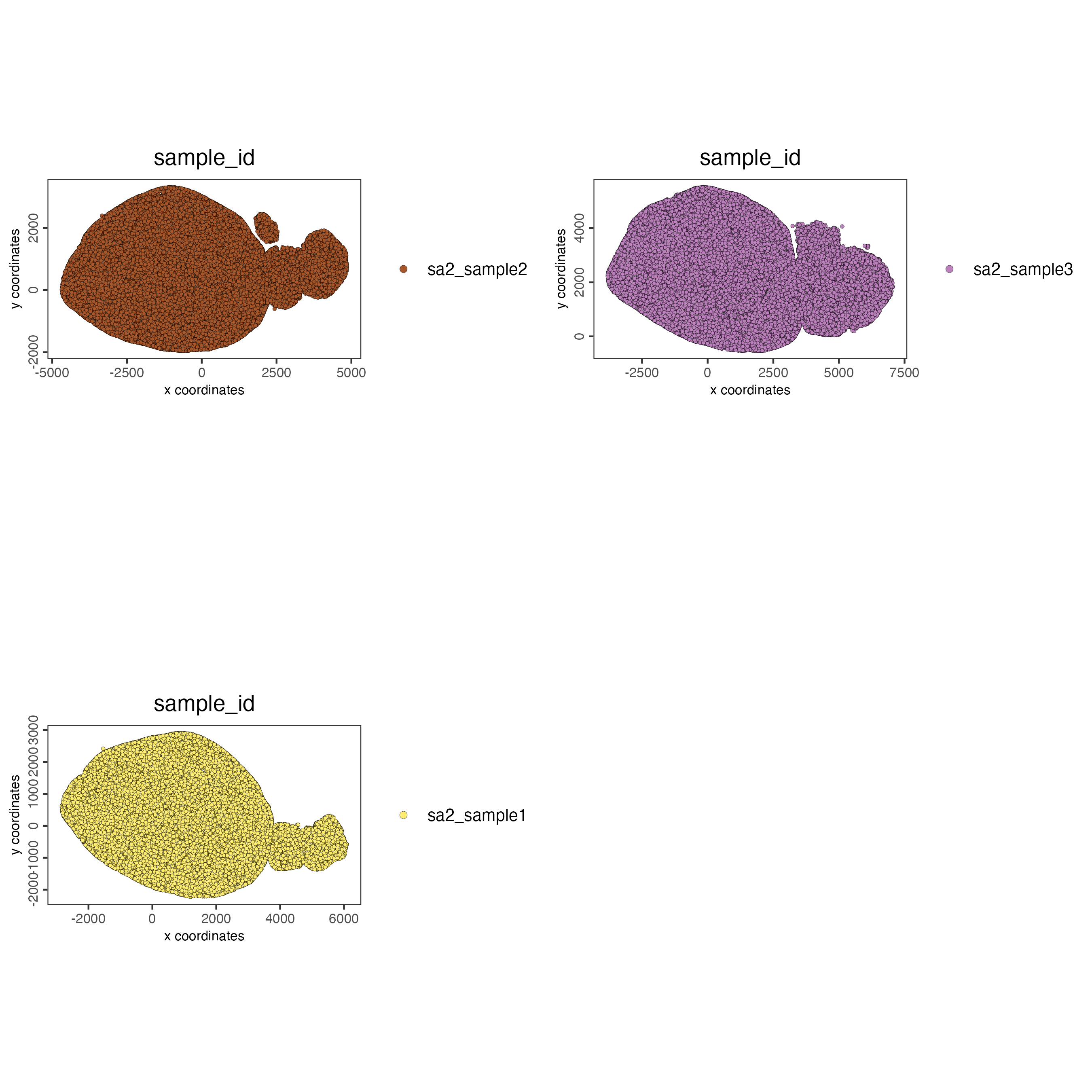
7 Subset data to keep only sample 1
g_s1 <- subsetGiotto(g,
                     cell_ids = cell_metadata[cell_metadata$sample_id == "sa2_sample1",]$cell_ID)
8 Quality control
Use the function addStatistics() to count the number of features per spot. The statistical information will be stored in the metadata table under the new column “nr_feats”. Then, use this column to visualize the number of features per spot across the sample.
filterDistributions(g_s1,
                    detection = "cells")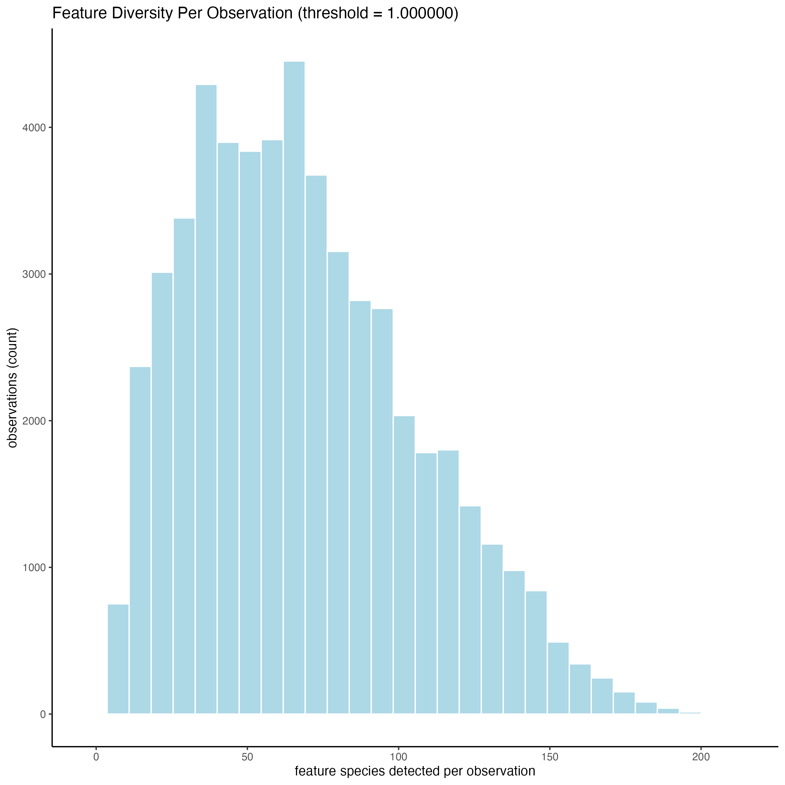
filterDistributions(g_s1,
                    detection = "feats")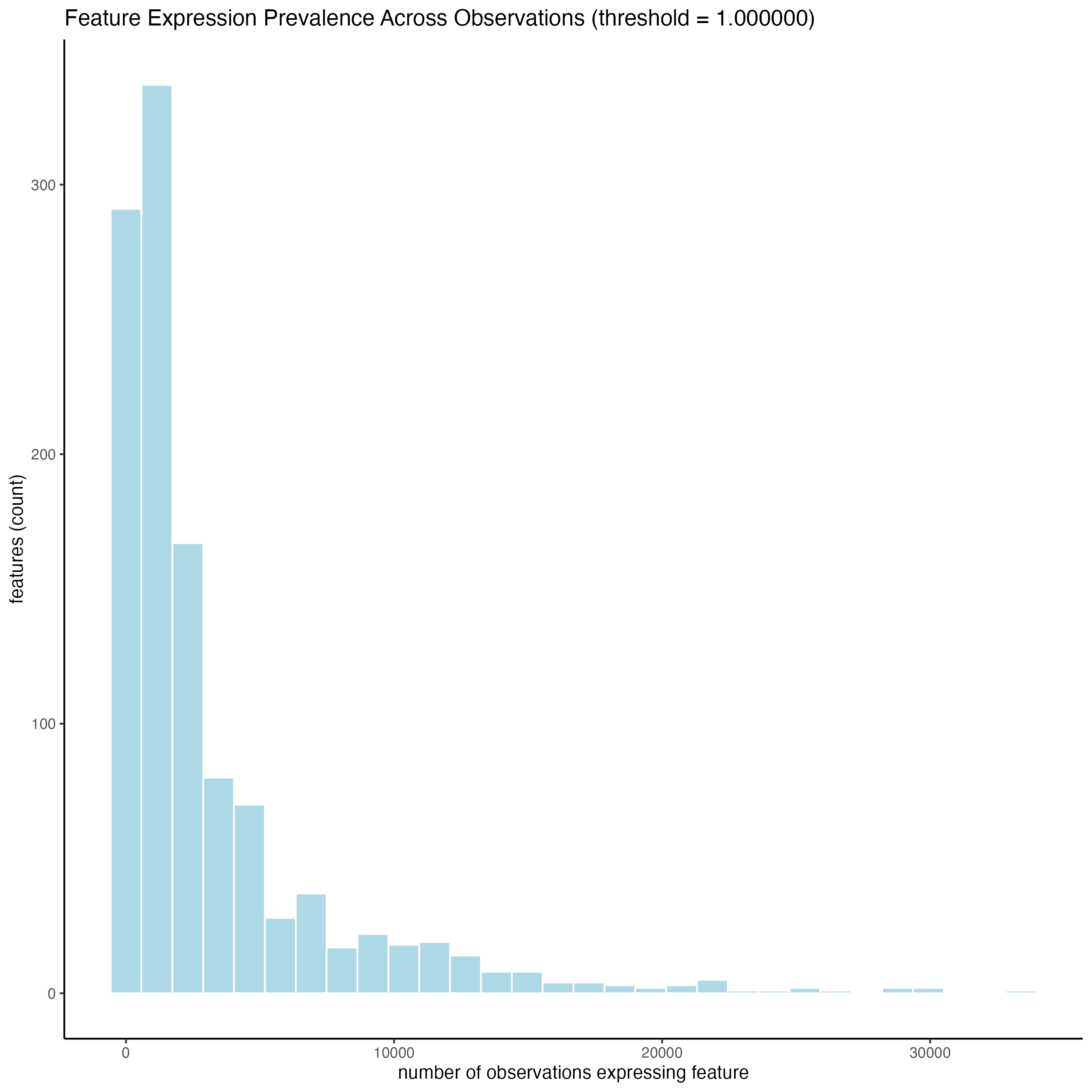
# add statistics
g_s1_stats <- addStatistics(g_s1,
                            expression_values = "raw")

spatPlot2D(g_s1_stats,
           cell_color = "nr_feats",
           color_as_factor = FALSE,
           point_size = 0.5)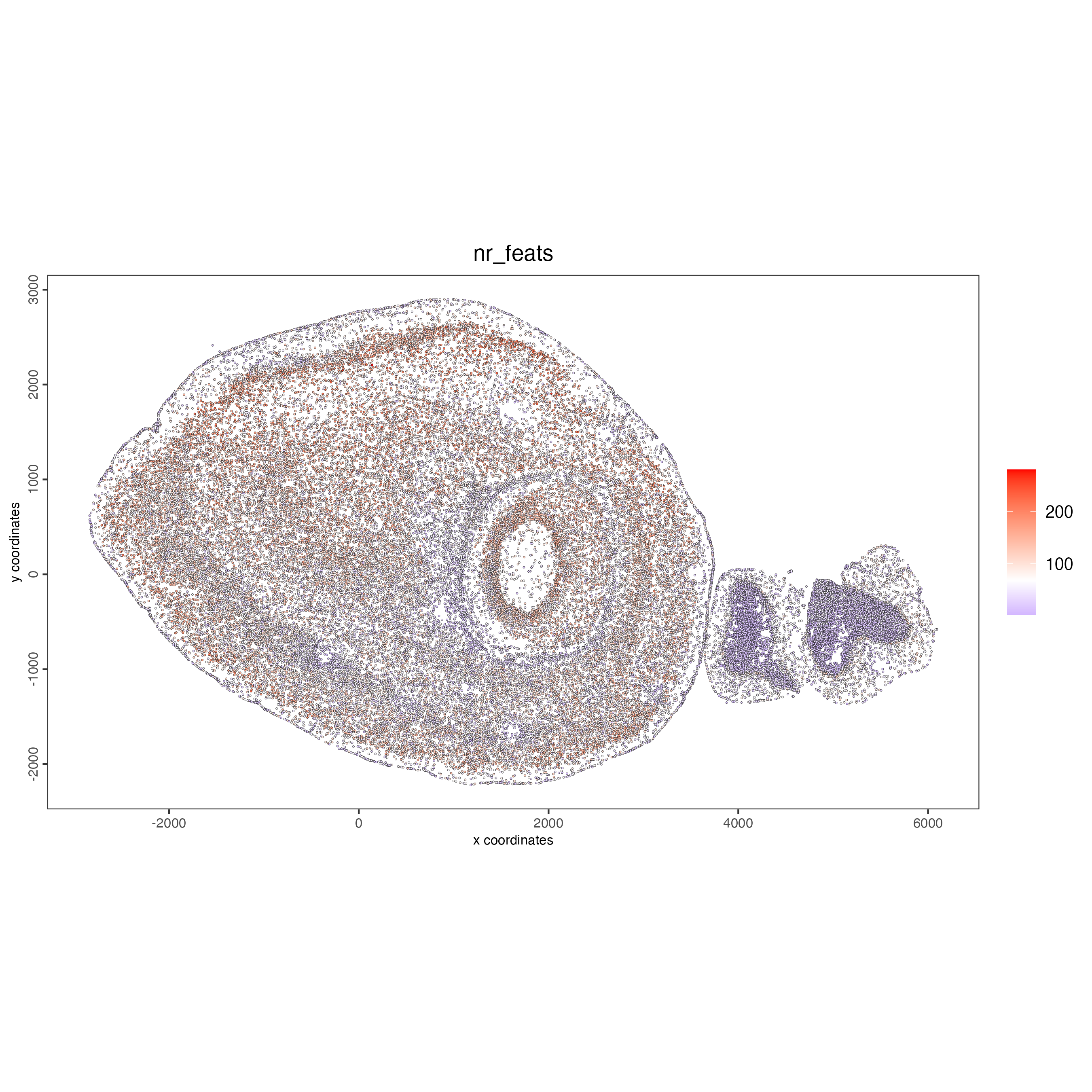
9 Filtering
Use the arguments feat_det_in_min_cells and min_det_feats_per_cell to set the minimal number of cells where an individual feature must be detected and the minimal number of features per spot/cell, respectively, to filter the giotto object. All the features and spots/cells under those thresholds will be removed from the sample.
g_s1 <- filterGiotto(g_s1,
                     min_det_feats_per_cell = 10,
                     feat_det_in_min_cells = 100)
10 Normalization
Use scalefactor to set the scale factor to use after library size normalization. The default value is 6000, but you can use a different one.
g_s1 <- normalizeGiotto(g_s1,
                        scalefactor = 6000,
                        verbose = TRUE)
11 Dimension reduction
11.1 PCA
Principal Components Analysis (PCA) is applied to reduce the dimensionality of gene expression data by transforming it into principal components, which are linear combinations of genes ranked by the variance they explain, with the first components capturing the most variance.
runPCA() will look for the previous calculation of highly variable features stored as a column in the feature metadata. If the HVF labels are not found in the Giotto object, runPCA() will use all the features available in the sample to calculate the Principal Components.
You can also use specific features for the Principal Components calculation by passing a vector of features in the “feats_to_use” argument.
Finally, create a scree plot to visualize the percentage of variance explained by each component.
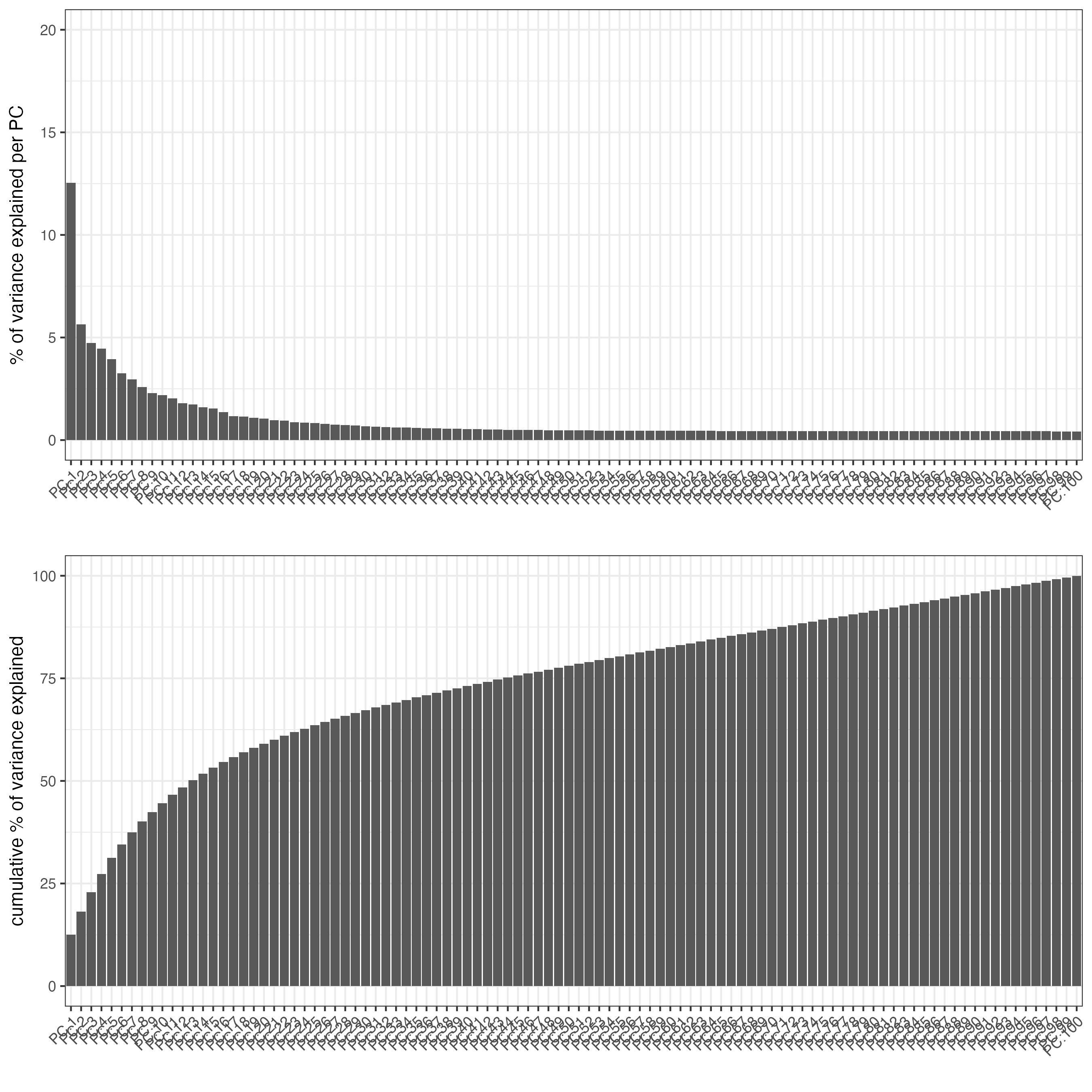
plotPCA(g_s1)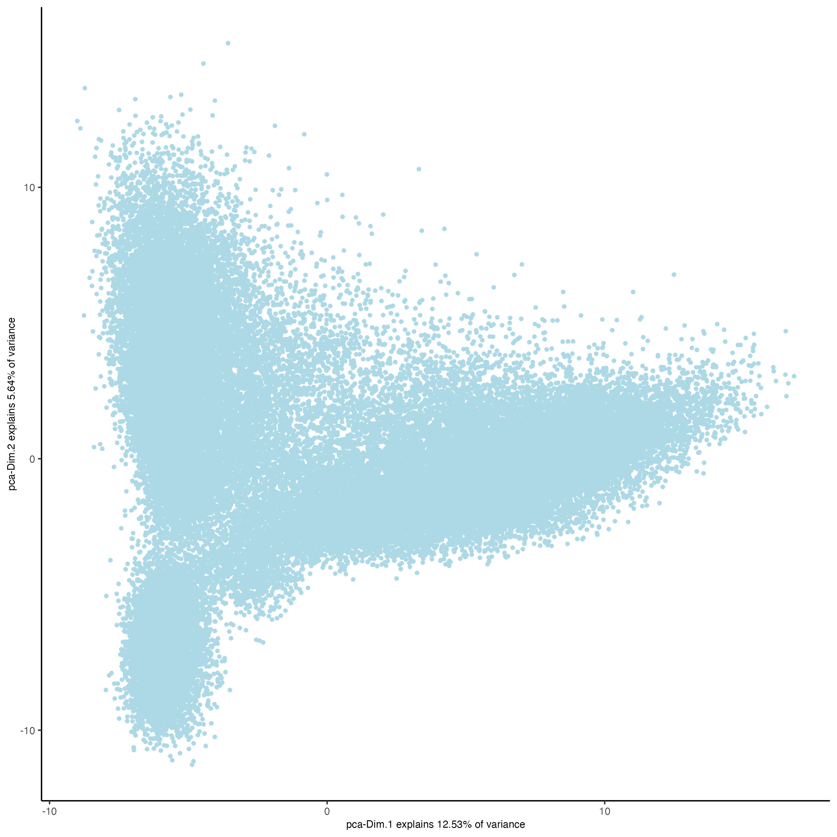
12 Calculate the nearest neighbors
In preparation for the clustering calculation, finding the spots/cells with similar expression patterns is needed. There are two methods available in Giotto:
- Create a sNN network (default) The shared Nearest Neighbor algorithm defines the similarity between a pair of points in terms of their shared nearest neighbors. That is, the similarity between two points is “confirmed” by their common (shared) near neighbors. If point A is close to point B and if they are both close to a set of points C then we can say that A and B are close with greater confidence since their similarity is “confirmed” by the points in set C. You can find more information about this method here. By default, createNearestNetwork() calculates 30 shared Nearest Neighbors for each spot/cell, but you can modify this number using the “k” parameter.
g_s1 <- createNearestNetwork(g_s1,
                             dimensions_to_use = 1:10,
k = 30)- Create a kNN network The K-Nearest Neighbors (kNN) algorithm operates on the principle of likelihood of similarity. It posits that similar data points tend to cluster near each other in space. You can find more information about this method here. By default, createNearestNetwork() finds the 30 K-Nearest Neighbors to each spot/cell, but you can modify this number using the “k” parameter.
g_s1 <- createNearestNetwork(g_s1,
                             dimensions_to_use = 1:10,
                             k = 30,
                             type = "kNN")
13 Leiden clustering
This algorithm is more complicated than the Louvain algorithm and have an accurate and fast result for the computation time. The Leiden algorithm consists of three phases. The first phase is the modularity optimization process, the second phase is the refinement of partition, and the third phase is the community aggregation process. This algorithm performs well on small, medium and large-scale networks. You can find more information about Louvain and Leiden clustering here.
This step may take some time to run
g_s1 <- doLeidenCluster(g_s1,
                        res = 1)
Visualization
plotPCA(g_s1,
        cell_color = "leiden_clus")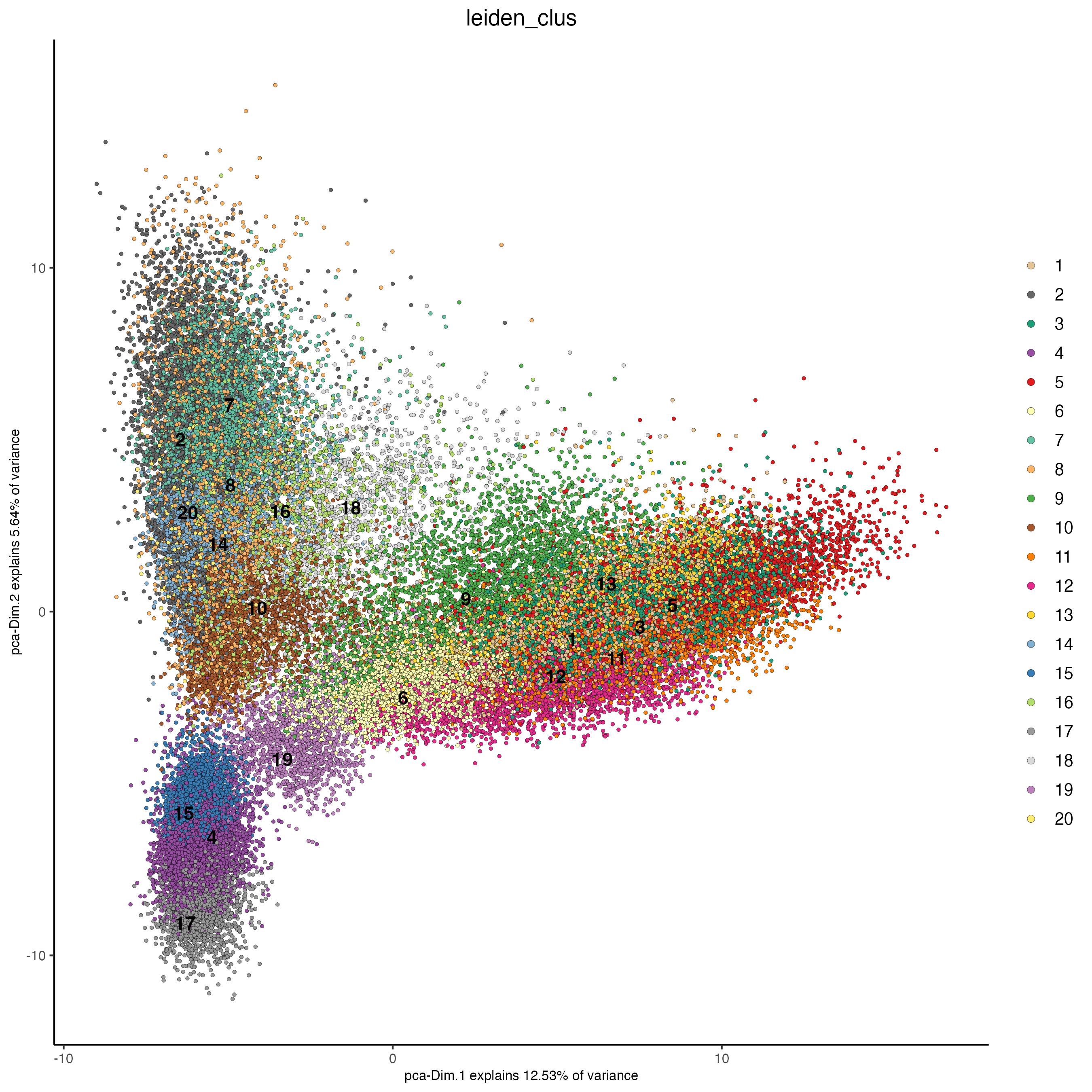
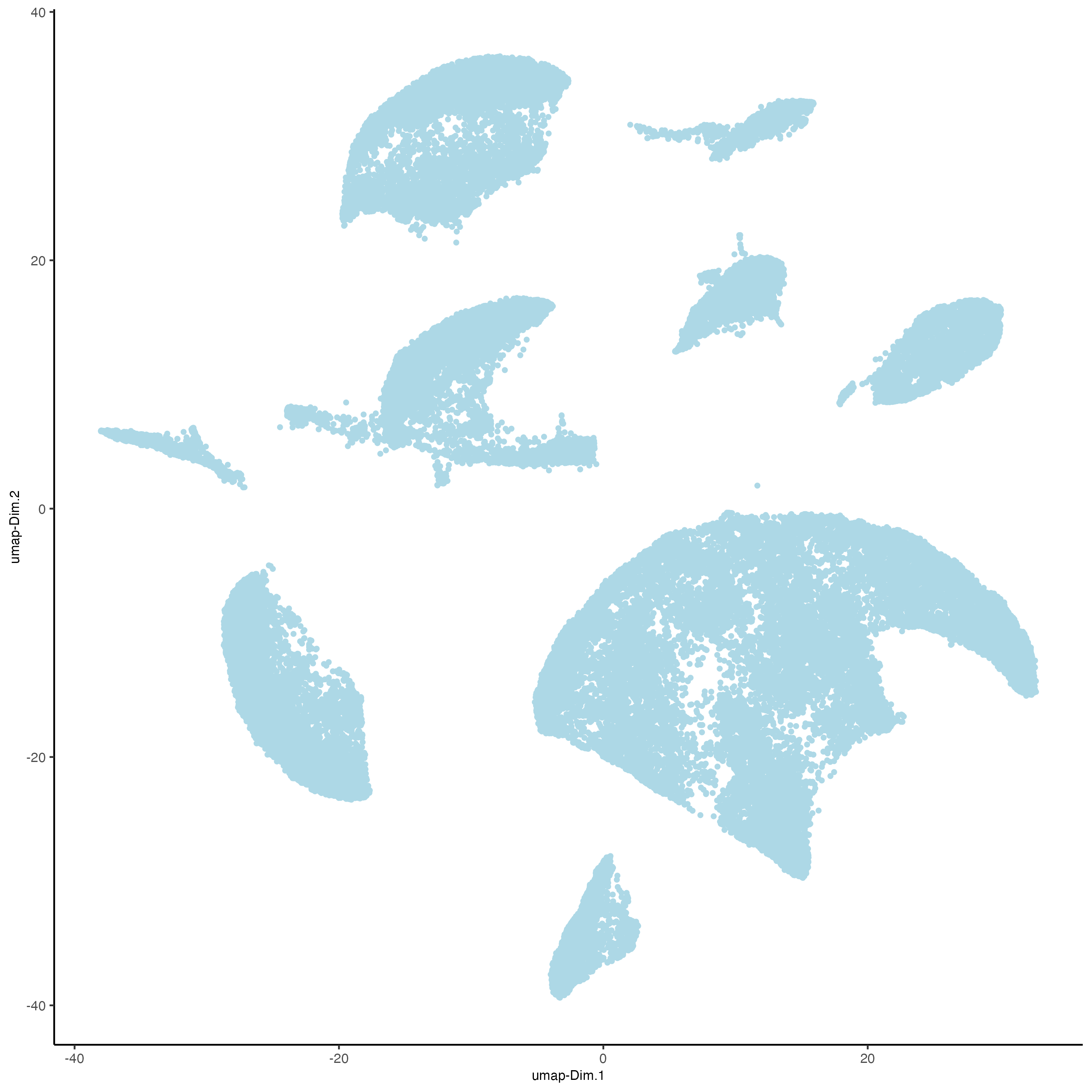
plotUMAP(g_s1,
         cell_color = "leiden_clus")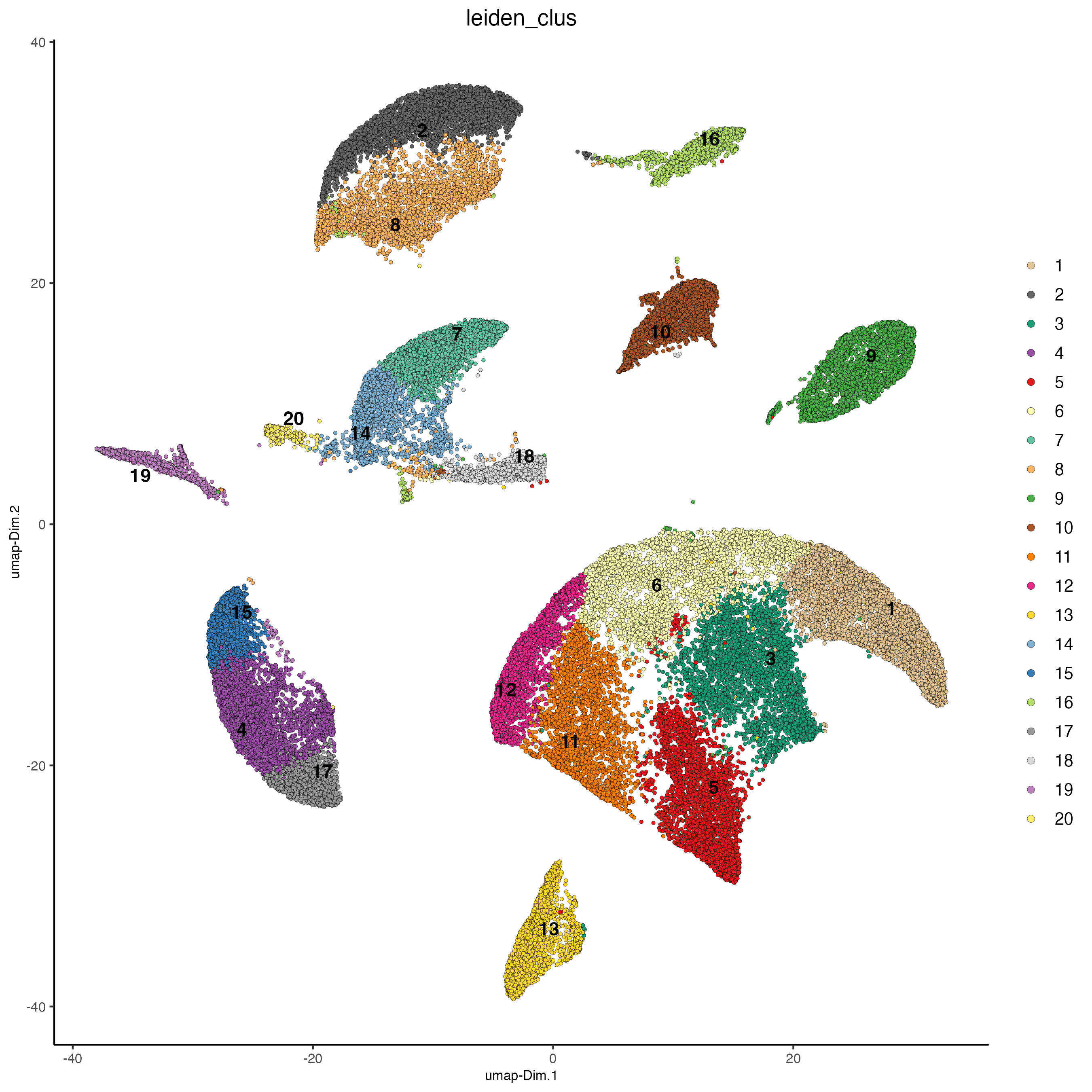
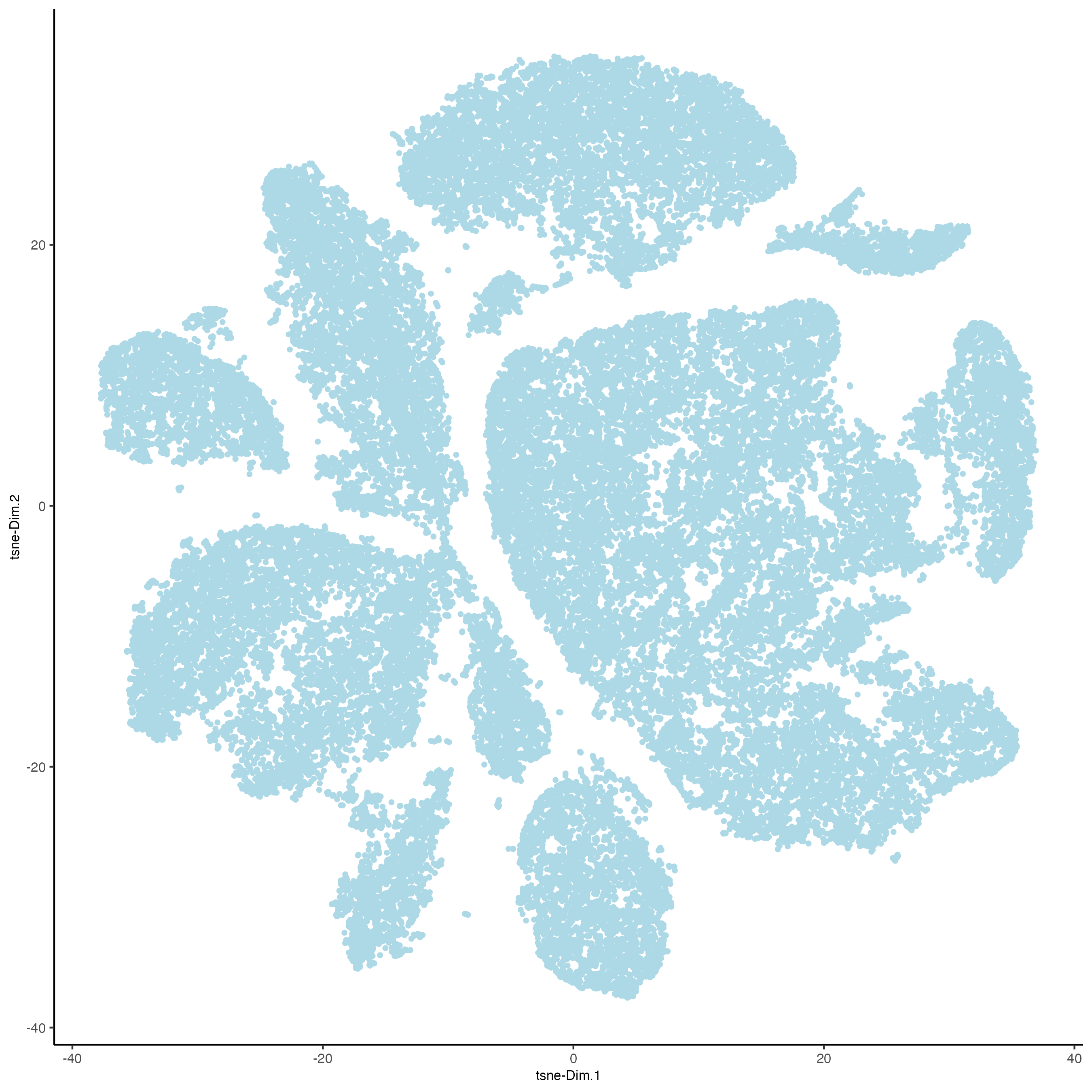
plotTSNE(g_s1,
         cell_color = "leiden_clus")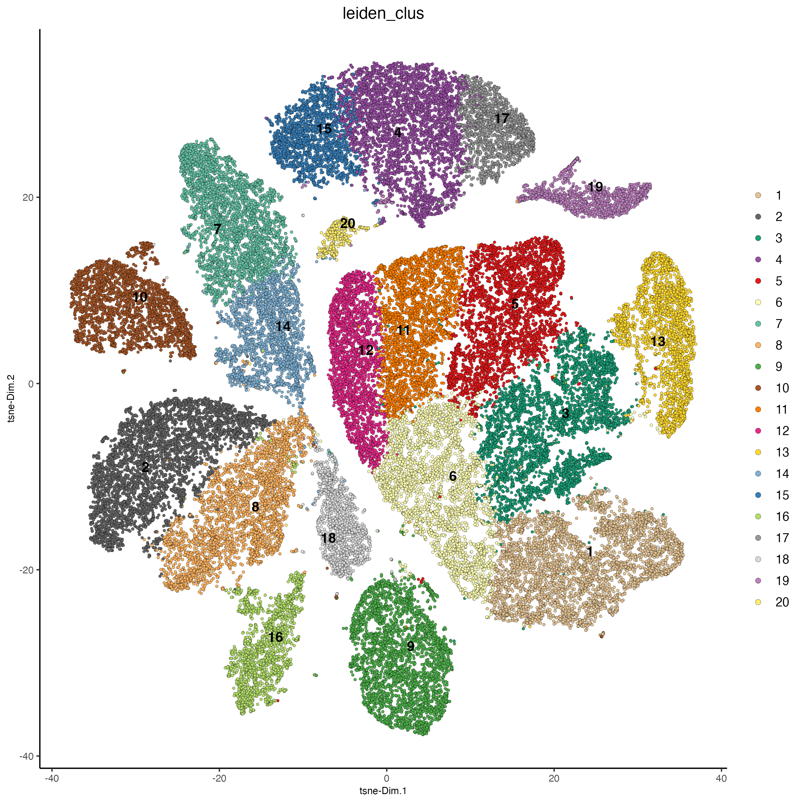
spatPlot2D(g_s1,
           cell_color = "leiden_clus",
           point_size = 1)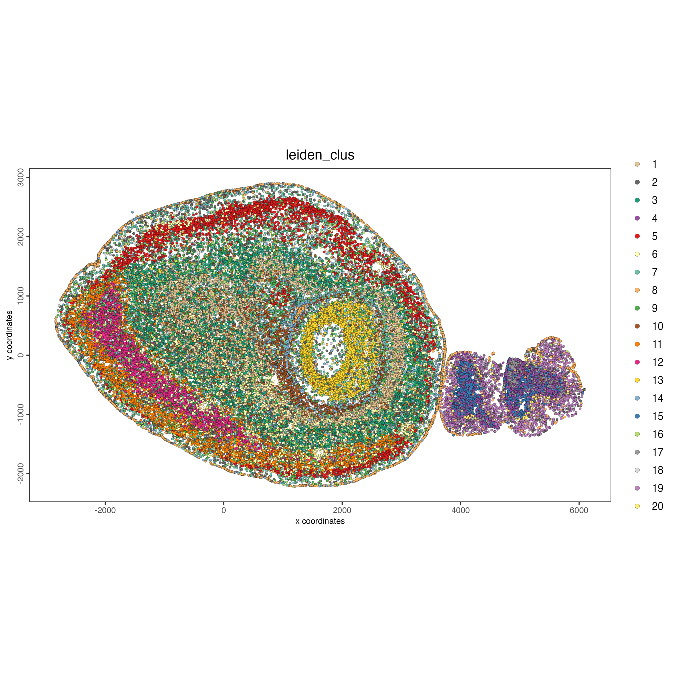
14 Finding differentially expressed genes
- The Gini method identifies genes that are very selectively expressed in a specific cluster, however not always expressed in all cells of that cluster. In other words, highly specific but not necessarily sensitive at the single-cell level.
Calculate the top marker genes per cluster using the gini method.
markers_gini <- findMarkers_one_vs_all(gobject = g_s1,
                                        method = "gini",
                                        expression_values = "normalized",
                                        cluster_column = "leiden_clus",
                                        min_feats = 10)

topgenes_gini <- markers_gini[, head(.SD, 3), by = "cluster"]$feats
Use the cluster IDs to create a heatmap with the normalized expression of the top-expressed genes per cluster.
plotMetaDataHeatmap(g_s1,
                    selected_feats = unique(topgenes_gini),
                    metadata_cols = "leiden_clus")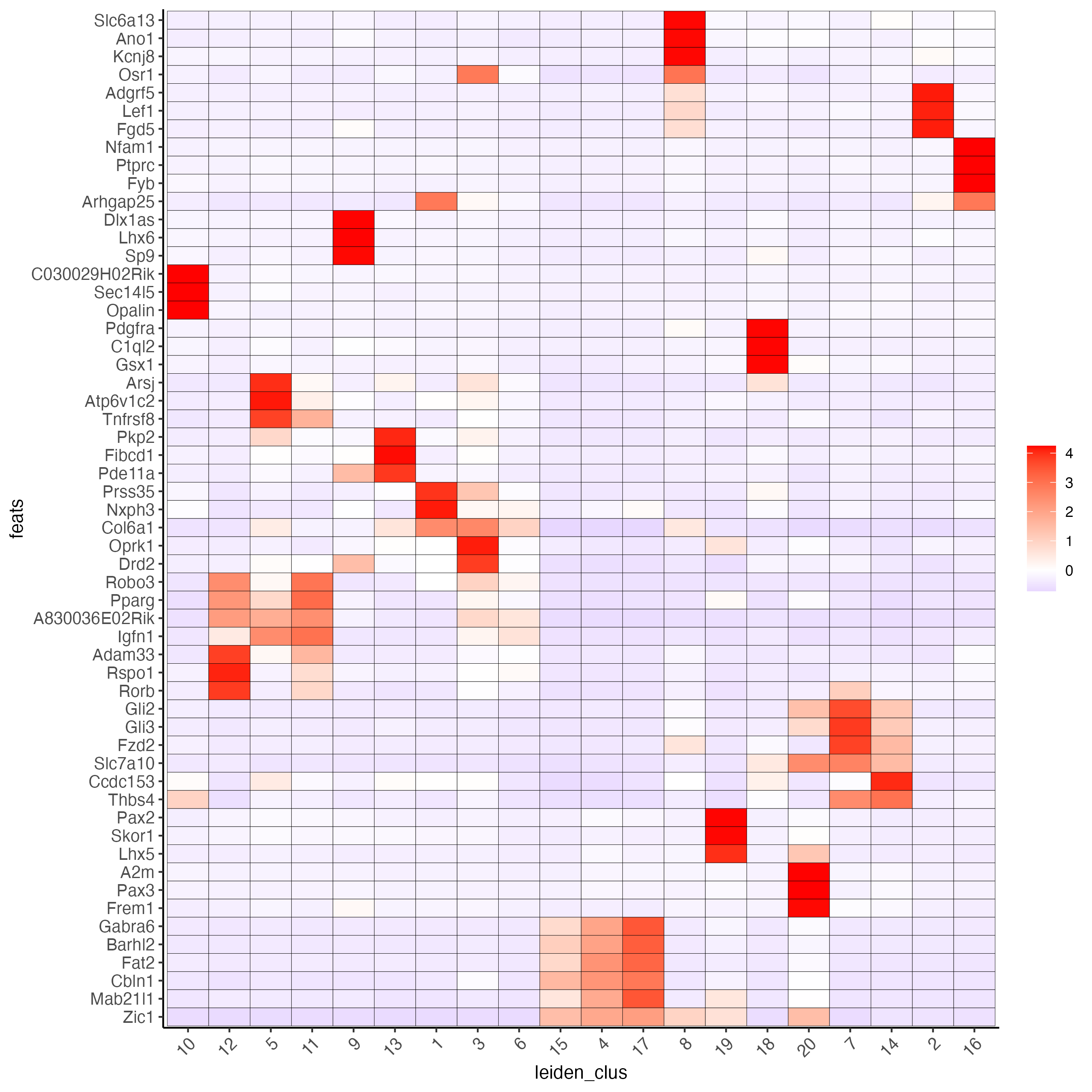
violinPlot(g_s1,
           feats = unique(topgenes_gini)[1:10],
           cluster_column = "leiden_clus",
           strip_text = 6,
           strip_position = "right")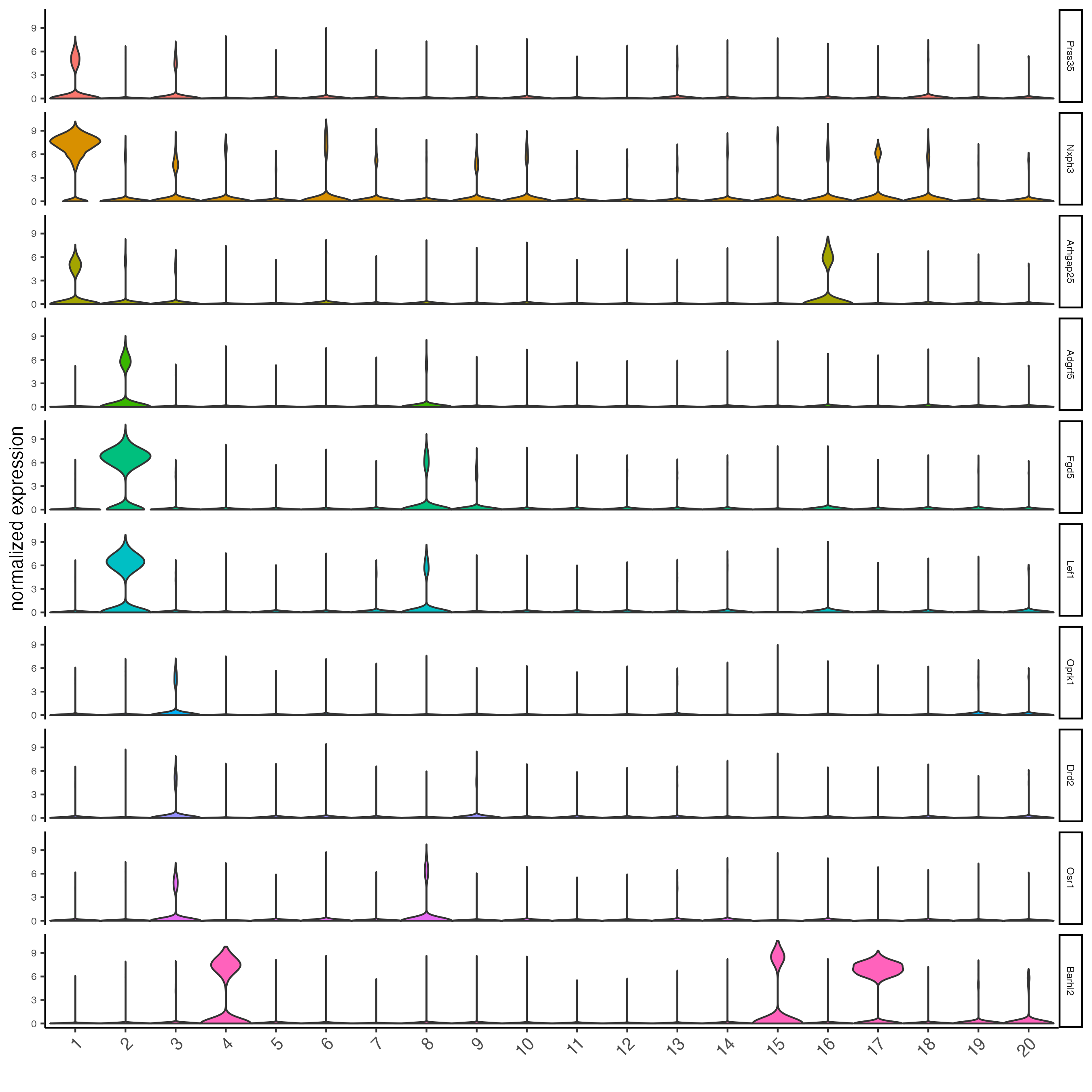
Visualize the scaled expression spatial distribution of the top-expressed genes across the sample.
dimFeatPlot2D(g_s1,
              expression_values = "scaled",
              feats = unique(topgenes_gini)[1:4],
              cow_n_col = 2,
              point_size = 1)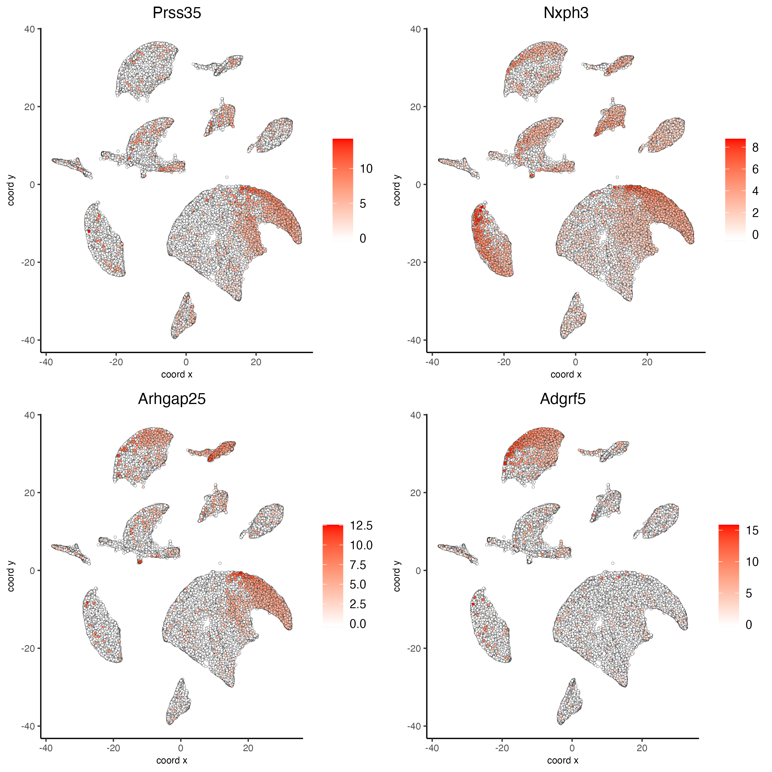
- The Scran method is preferred for robust differential expression analysis, especially when addressing technical variability or differences in sequencing depth across spatial locations.
markers_scran <- findMarkers_one_vs_all(gobject = g_s1,
                                        method = "scran",
                                        expression_values = "normalized",
                                        cluster_column = "leiden_clus",
                                        min_feats = 10)

topgenes_scran <- markers_scran[, head(.SD, 3), by = "cluster"]$feats
Use the cluster IDs to create a heatmap with the normalized expression of the top-expressed genes per cluster.
plotMetaDataHeatmap(g_s1,
                    selected_feats = unique(topgenes_scran),
                    metadata_cols = "leiden_clus")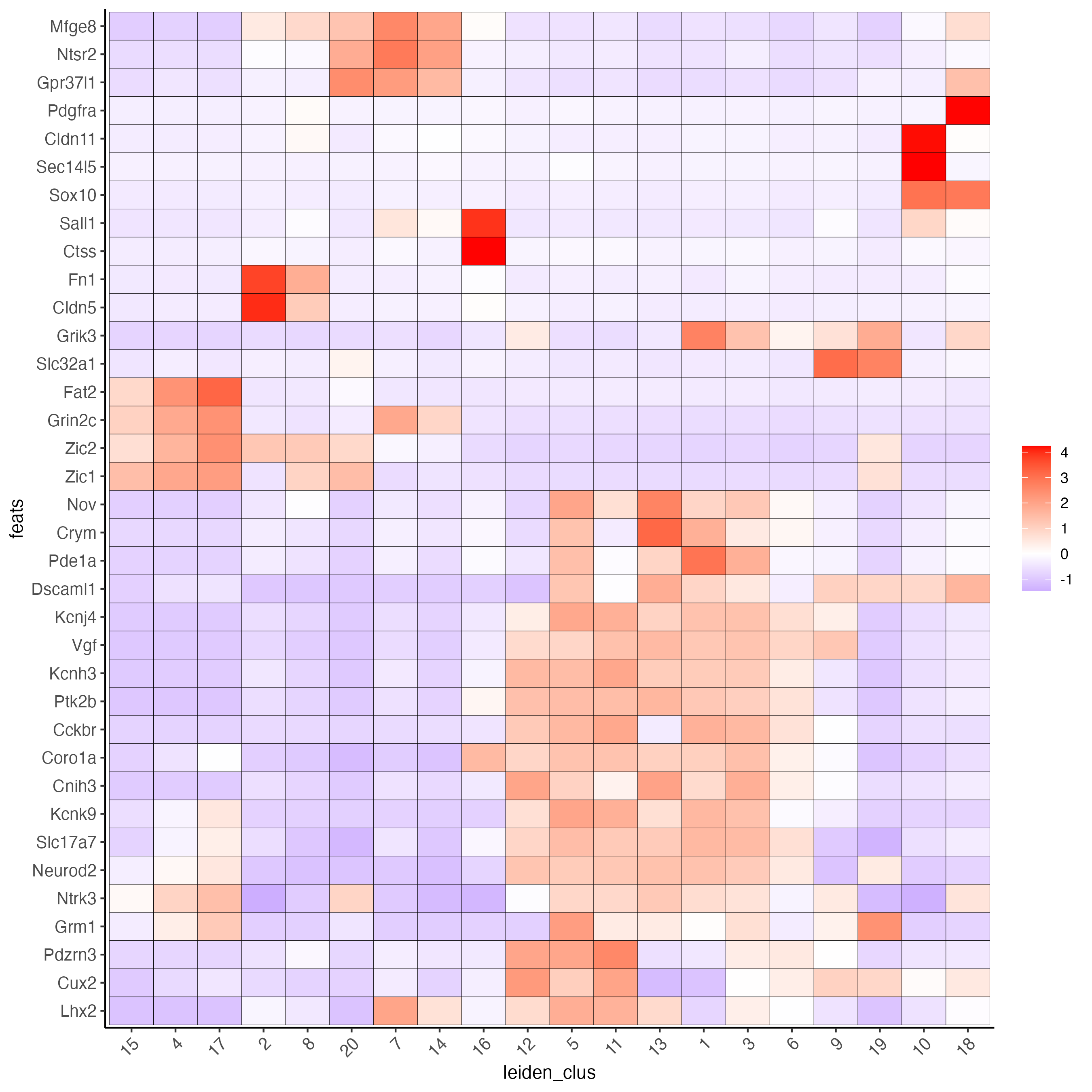
violinPlot(g_s1,
           feats = unique(topgenes_scran)[1:10],
           cluster_column = "leiden_clus",
           strip_text = 6,
           strip_position = "right")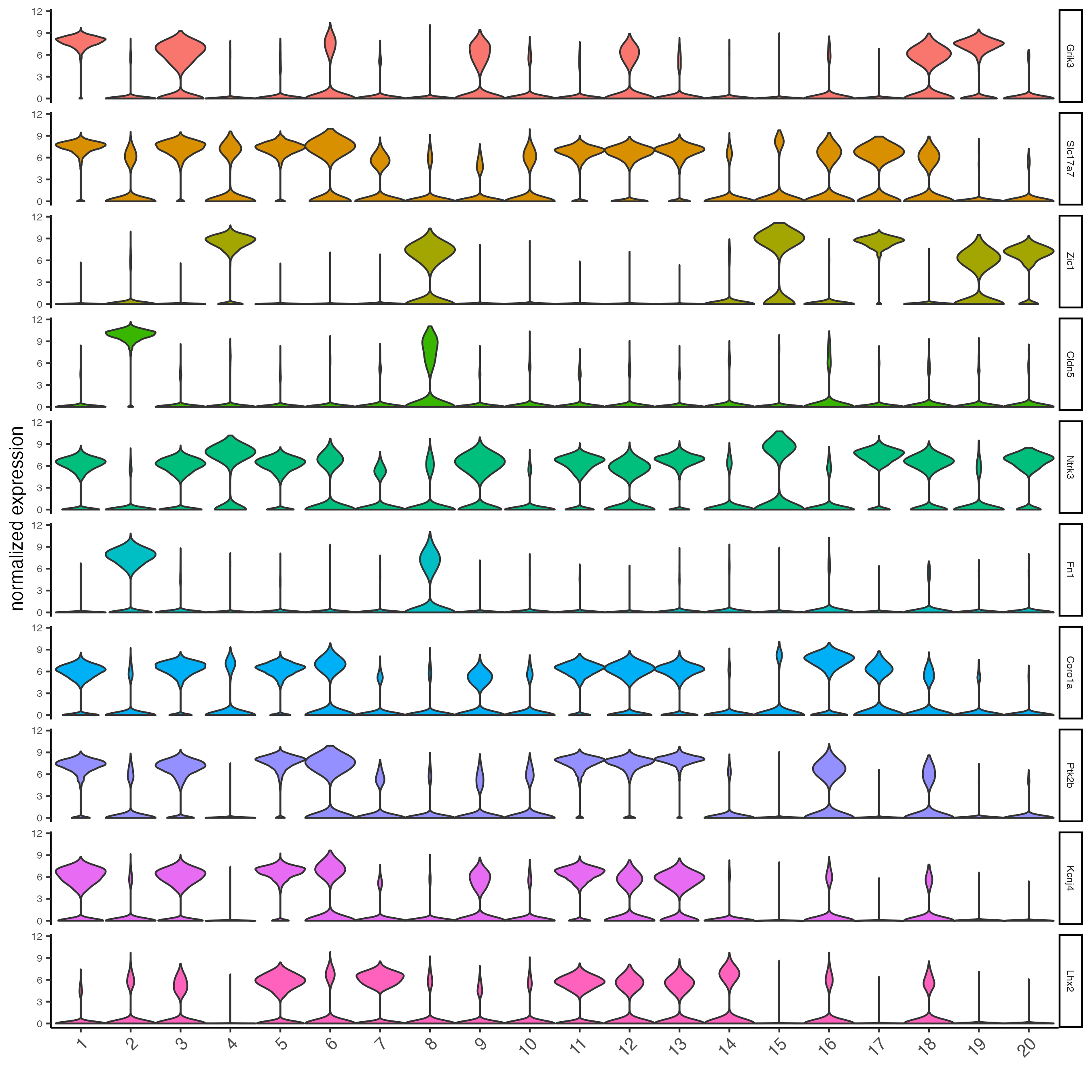
Visualize the scaled expression spatial distribution of the top-expressed genes across the sample.
dimFeatPlot2D(g_s1,
              expression_values = "scaled",
              feats = unique(topgenes_scran)[1:4],
              cow_n_col = 2,
              point_size = 1)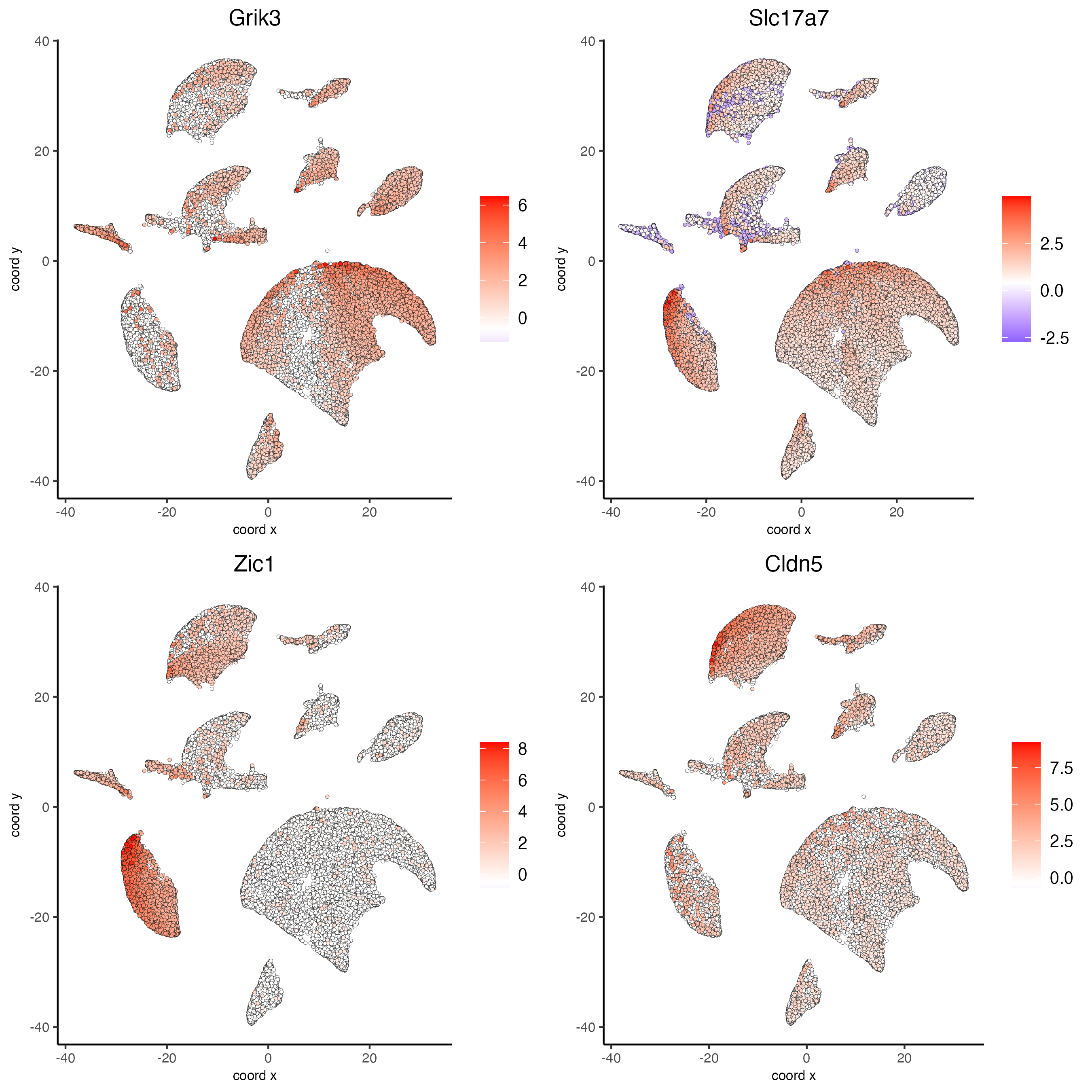
15 Finding spatial genes
When having the spatial location of each spot/cell, you can look for genes that follow and share particular spatial distributions.
15.1 Create a spatial network
createSpatialNetwork() creates a spatial network connecting single-cells based on their physical distance to each other. There are two methods available: Delaunay and kNN. For the Delaunay method, neighbors will be decided by Delaunay triangulation and a maximum distance criterion. For the kNN method, the number of neighbors can be determined by k, or the maximum distance from each cell with or without setting a minimum k for each cell.
g_s1 <- createSpatialNetwork(gobject = g_s1,
                             method = "kNN",
                             k = 6,
                             maximum_distance_knn = 400,
                             name = "spatial_network")

spatPlot2D(gobject = g_s1,
           point_size = 0.5,
           show_network = TRUE,
           network_color = "blue",
           spatial_network_name = "spatial_network")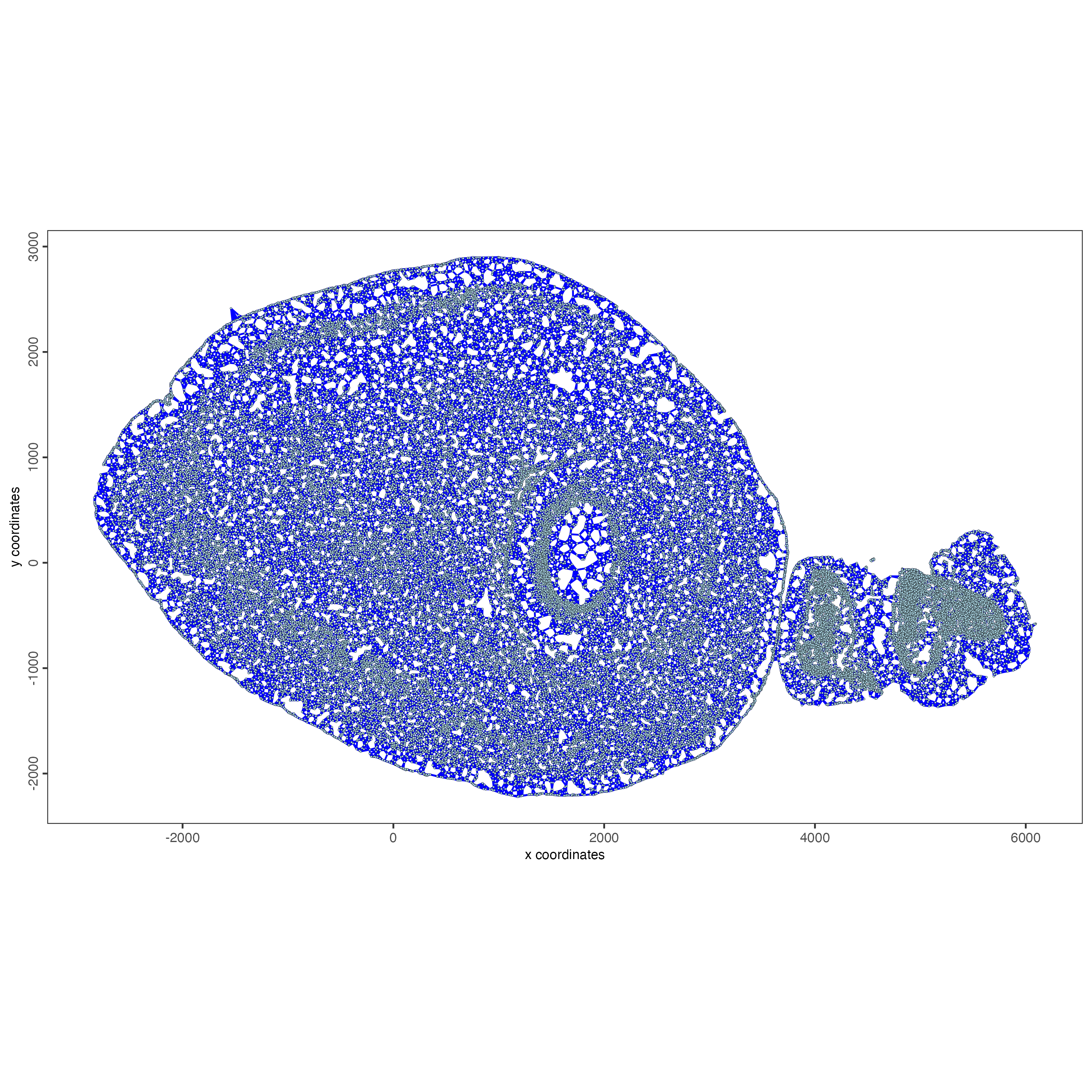
15.2 Find spatial genes
Use the rank binarization to rank genes on the spatial dataset depending on whether they exhibit a spatial pattern location or not. This step may take a few minutes to run.
ranktest <- binSpect(g_s1,
                     bin_method = "rank",
                     calc_hub = TRUE,
                     hub_min_int = 5,
                     spatial_network_name = "spatial_network")
Plot the scaled expression of genes with the highest probability of being spatial genes.
spatFeatPlot2D(g_s1,
               expression_values = "scaled",
               feats = ranktest$feats[1:6],
               cow_n_col = 2,
               point_size = 1)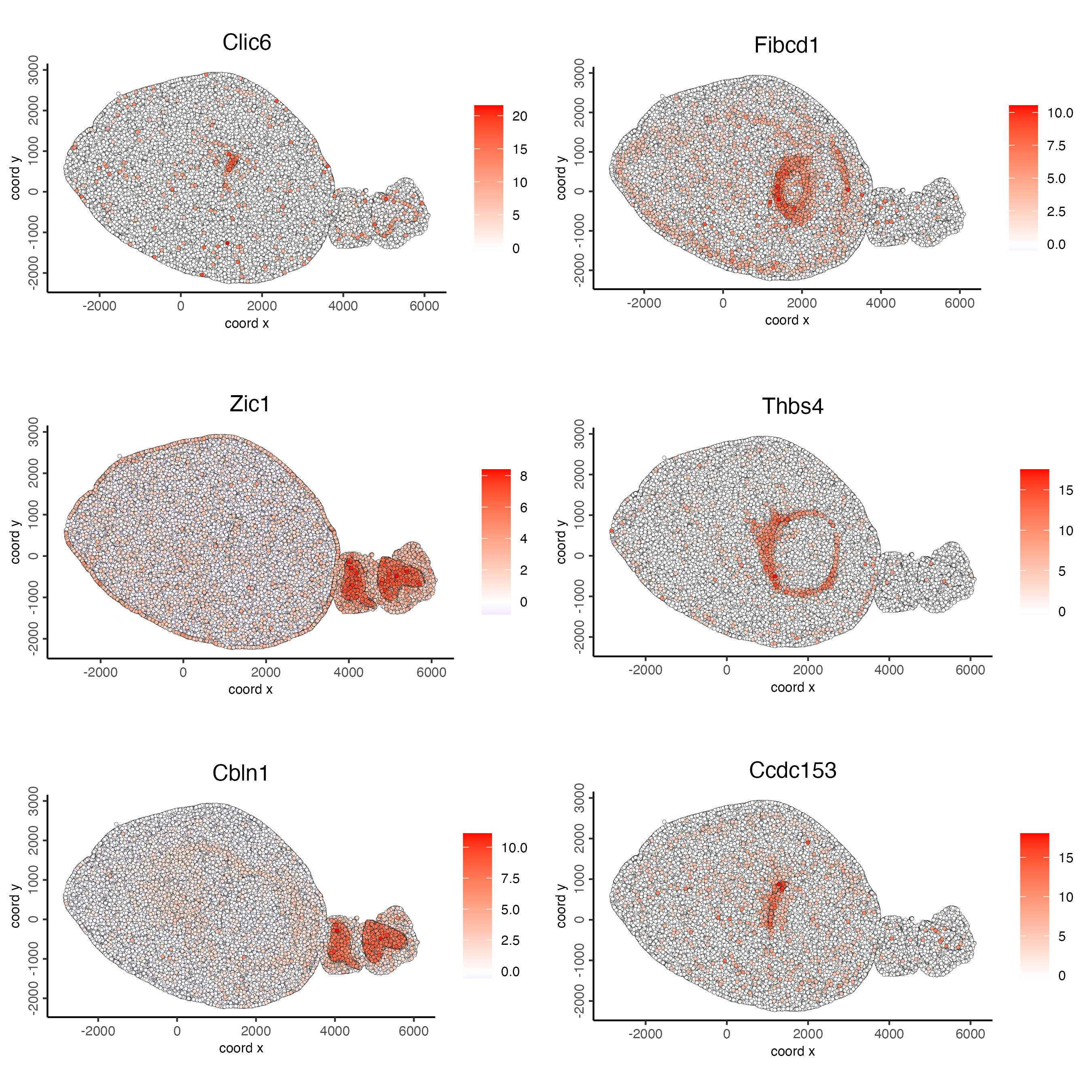
16 Spatial Co-Expression modules
Once we have found spatial genes, we can group those genes with similar spatial patterns into co-expression modules.
- Cluster the top 100 spatial genes into 5 clusters
ext_spatial_genes <- ranktest[1:100,]$feats- Use detectSpatialCorGenes() to calculate pairwise distances between genes.
spat_cor_netw_DT <- detectSpatialCorFeats(g_s1,
                                          method = "network",
                                          spatial_network_name = "spatial_network",
subset_feats = ext_spatial_genes)- Cluster spatial genes.
spat_cor_netw_DT <- clusterSpatialCorFeats(spat_cor_netw_DT,
                                           name = "spat_netw_clus",
k = 5)- Rank spatial correlated clusters and show genes for selected clusters.
netw_ranks <- rankSpatialCorGroups(g_s1,
                                   spatCorObject = spat_cor_netw_DT,
                                   use_clus_name = "spat_netw_clus")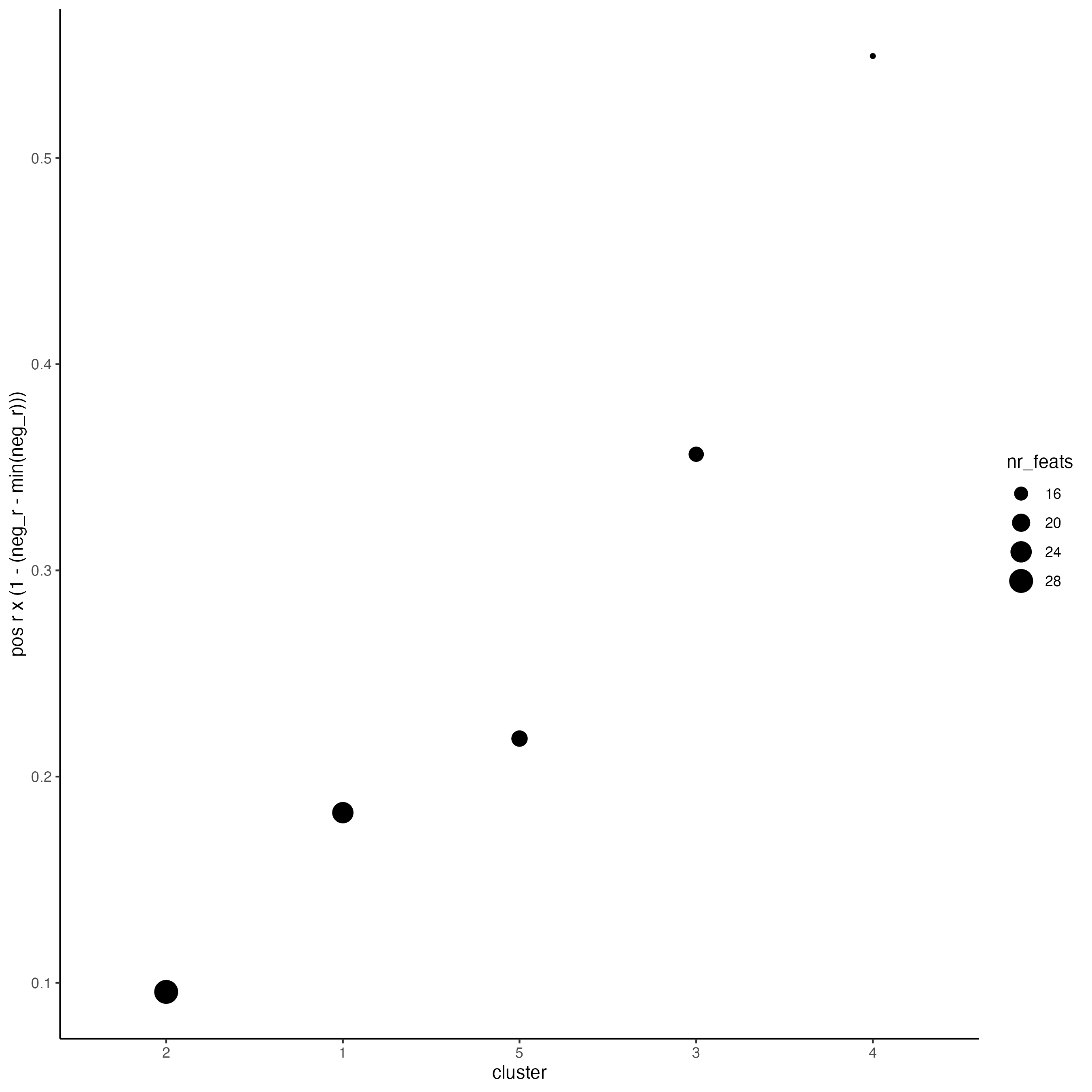
- Plot the correlation and number of spatial genes in each cluster.
top_netw_spat_cluster <- showSpatialCorFeats(spat_cor_netw_DT,
                                             use_clus_name = "spat_netw_clus",
                                             selected_clusters = 6,
show_top_feats = 1)- Create the metagene enrichment score per co-expression cluster.
cluster_genes_DT <- showSpatialCorFeats(spat_cor_netw_DT,
                                        use_clus_name = "spat_netw_clus",
                                        show_top_feats = 1)

cluster_genes <- cluster_genes_DT$clus
names(cluster_genes) <- cluster_genes_DT$feat_ID

g_s1 <- createMetafeats(g_s1,
                        feat_clusters = cluster_genes,
name = "cluster_metagene")- Plot the spatial distribution of the metagene enrichment scores of each spatial co-expression cluster.
spatCellPlot(g_s1,
             spat_enr_names = "cluster_metagene",
             cell_annotation_values = netw_ranks$clusters,
             point_size = 1,
             cow_n_col = 2)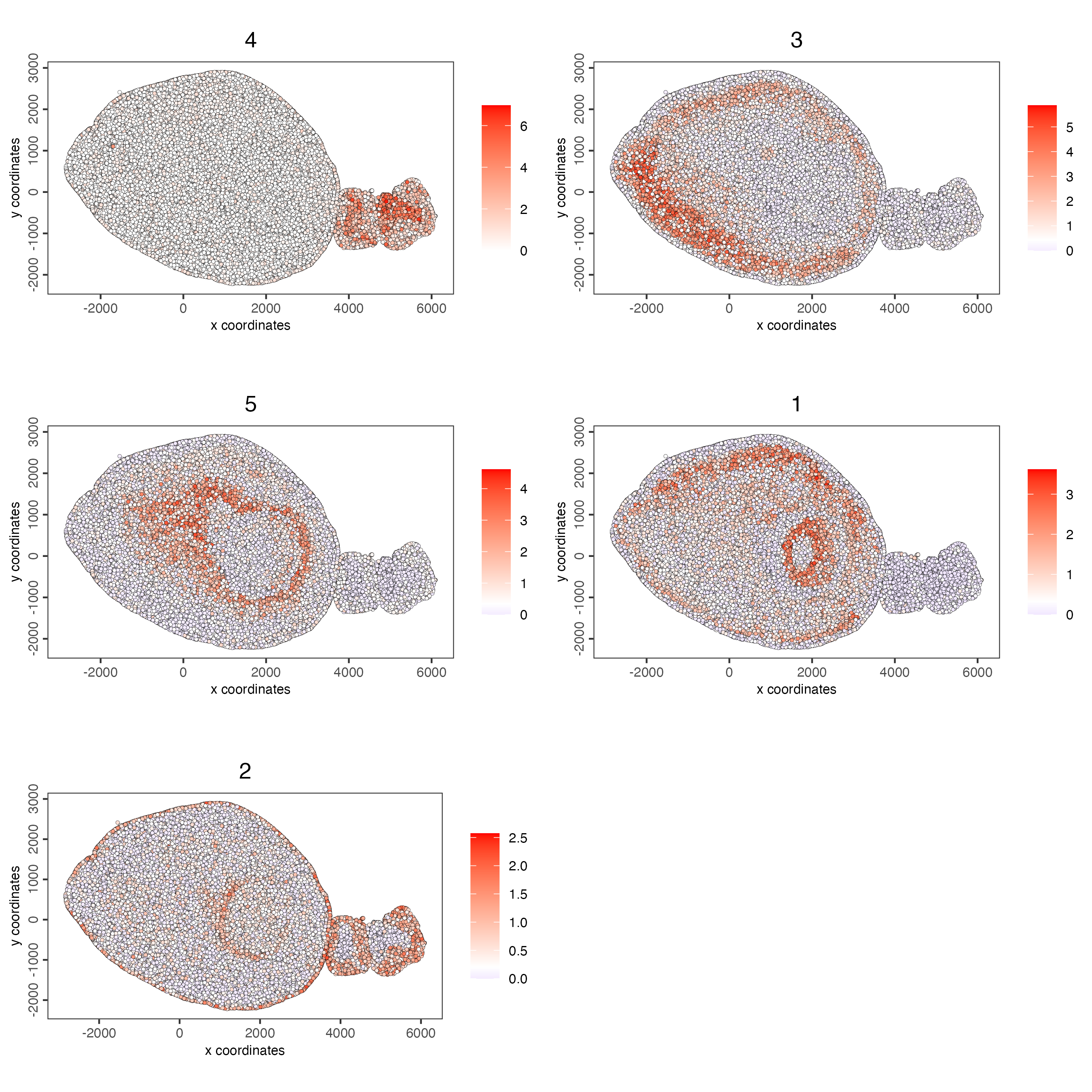
17 Spatially informed clusters
Once we have identified spatial genes, we can use them to re-calculate the clusters based only on the expression information that follows spatial patterns.
spatial_genes <- ranktest[1:200,]$feats17.1 Re-calculate the clustering
Use the spatial genes to calculate again the principal components, umap, network and clustering.
g_s1 <- runPCA(gobject = g_s1,
               feats_to_use = spatial_genes,
               name = "custom_pca",
               ncp = 50)

screePlot(g_s1,
          dim_reduction_name = "custom_pca")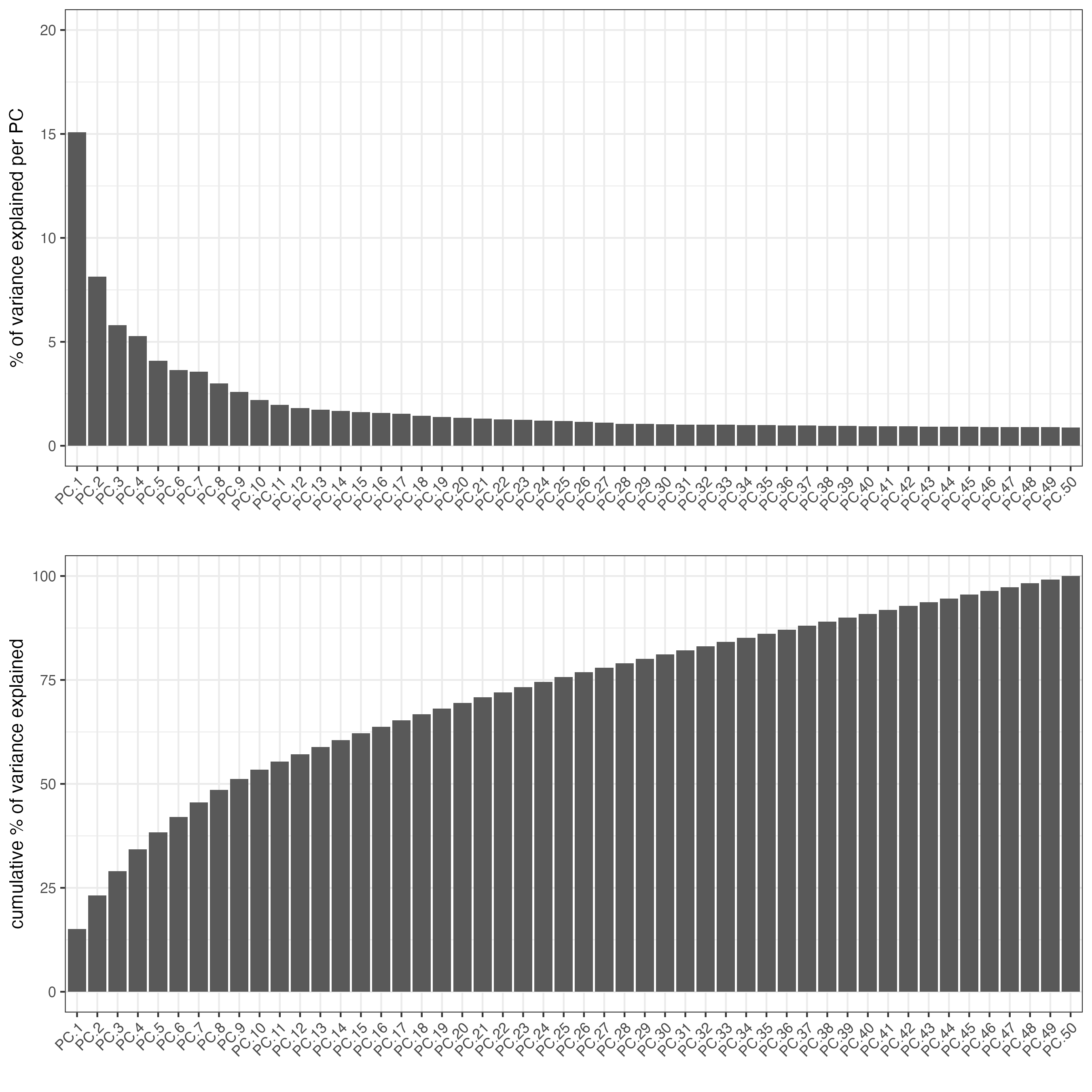
g_s1 <- runUMAP(g_s1,
                dim_reduction_name = "custom_pca",
                dimensions_to_use = 1:20,
                name = "custom_umap")

g_s1 <- createNearestNetwork(gobject = g_s1,
                             dim_reduction_name = "custom_pca",
                             dimensions_to_use = 1:20,
                             k = 5,
                             name = "custom_NN")

g_s1 <- doLeidenCluster(gobject = g_s1,
                        network_name = "custom_NN",
                        resolution = 0.1,
                        name = "custom_leiden")

plotPCA(g_s1,
        dim_reduction_name = "custom_pca",
        cell_color = "custom_leiden")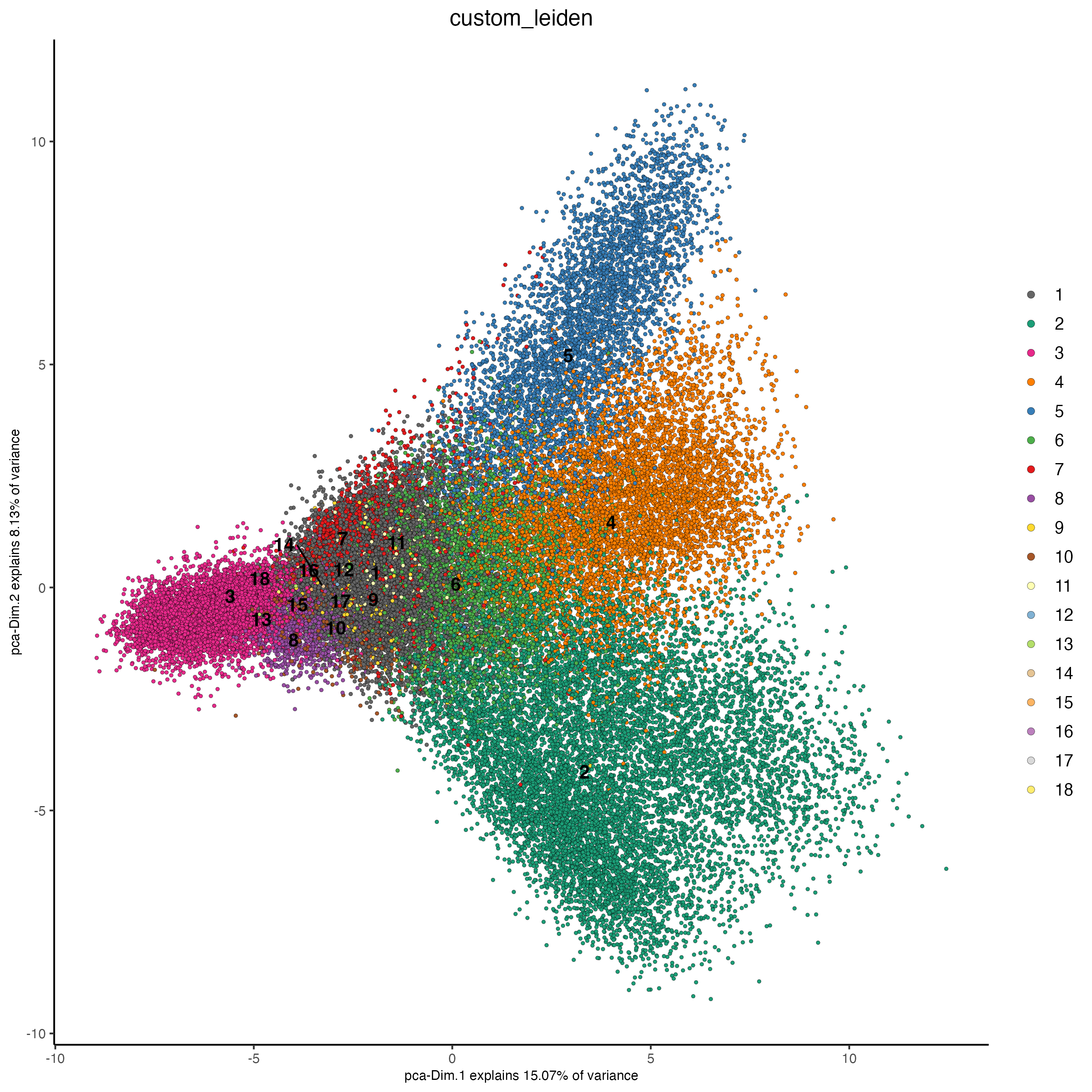
plotUMAP(g_s1,
        dim_reduction_name = "custom_umap",
        cell_color = "custom_leiden")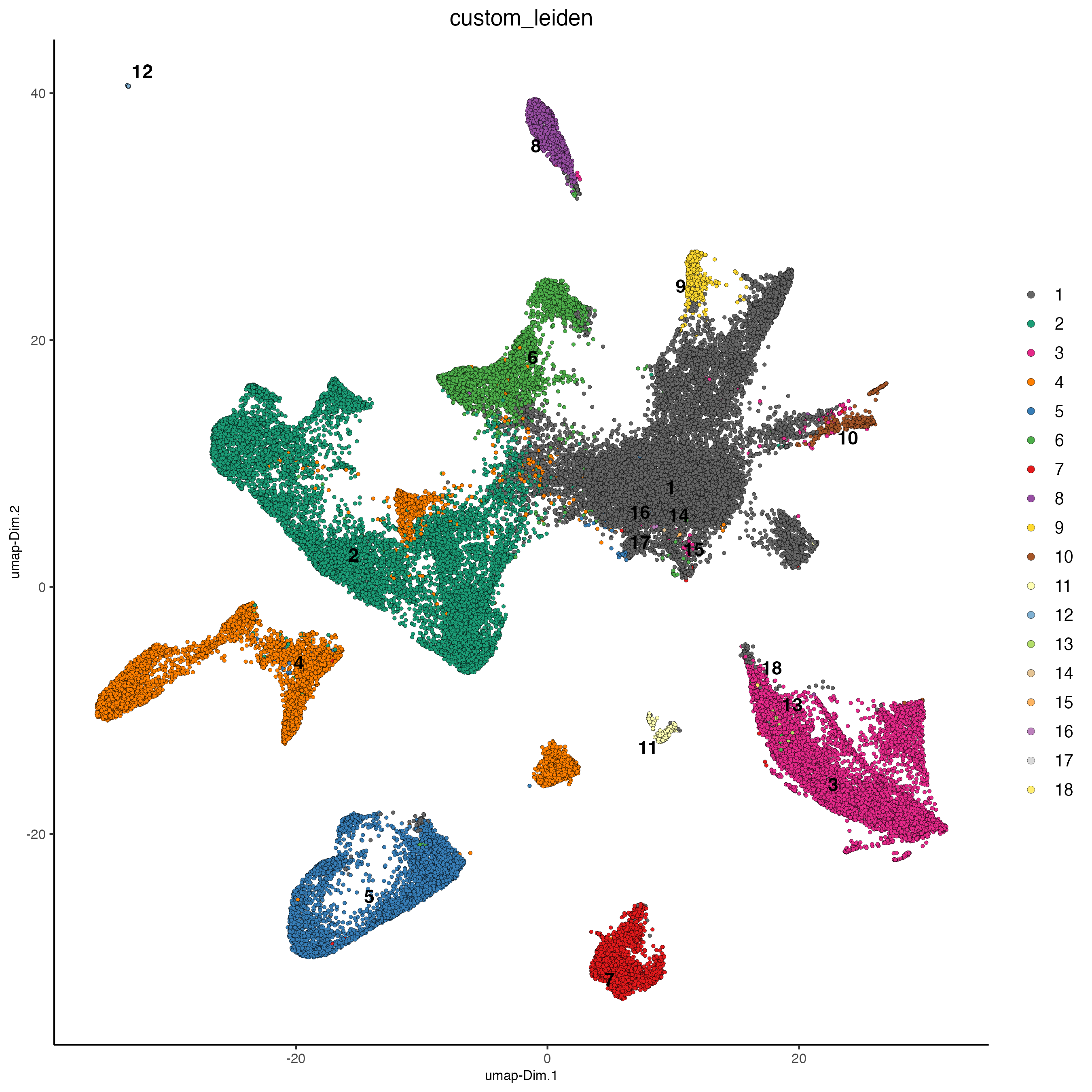
spatPlot2D(g_s1,
           cell_color = "custom_leiden",
           point_size = 1)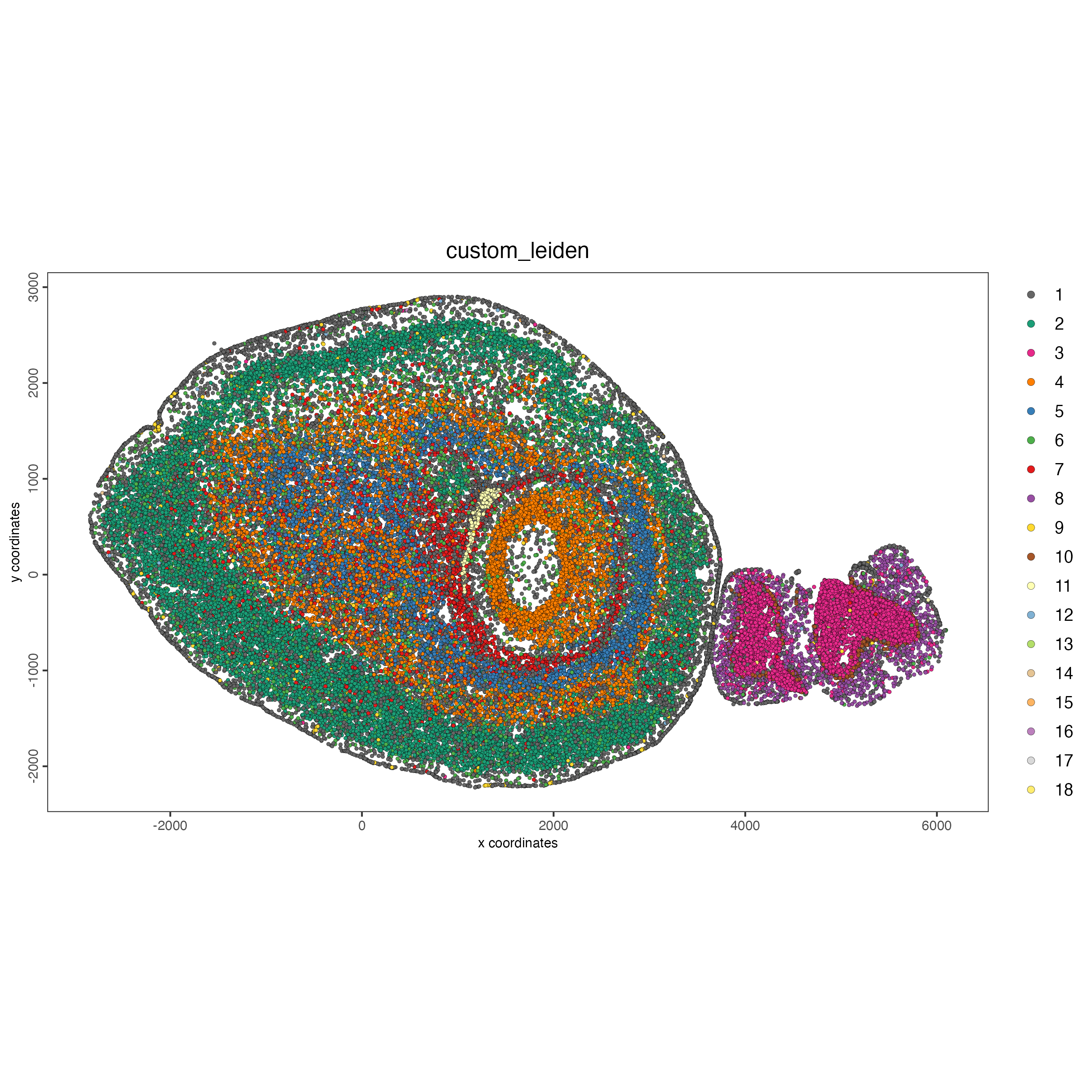
18 Integration with scRNAseq data
Single-cell datasets lack spatial context however, they tend to have clearer separation between clusters, making it easier to see which clusters correspond to which cell types. This dataset comes from the Mouse Brain Atlas and can be downloaded using GiottoData. We can use the single-cell data to identify cell types, then transfer those labels to the MERFISH data.
18.1 Download the single-cell dataset
GiottoData::getSpatialDataset(dataset = "scRNA_mouse_brain",
                              directory = "./")
18.2 Read scRNAseq data
sc_expression <- "brain_sc_expression_matrix.txt.gz"
sc_metadata <-  "brain_sc_metadata.csv"

instructions <- createGiottoInstructions(save_plot = TRUE,
                                         show_plot = FALSE,
                                         return_plot = FALSE,
                                         python_path = NULL)

giotto_SC <- createGiottoObject(expression = sc_expression,
                                instructions = instructions)
18.3 Create a joined spatial and single cell giotto object to transfer the cell type labels
# match features
ufids <- intersect(featIDs(g_s1), featIDs(giotto_SC)) # 1126 feats in common

# strip gobjects down to remove incompatible elements in join
sc_join <- giotto() |>
    setGiotto(giotto_SC[[c("expression", "spatial_locs"), "raw"]])

cell_metadata <- data.table::fread(sc_metadata)
sc_join <- addCellMetadata(sc_join,
                           new_metadata = cell_metadata[, c("Class", "Subclass")])

spatial_join <- giotto() |>
    setGiotto(g_s1[[c("expression", "spatial_locs"), "raw", spat_unit = "cell"]])

j <- joinGiottoObjects(
    list(sc_join[ufids], spatial_join[ufids]),
    gobject_names = c("sc", "merfish")
)
instructions(j) <- instructions
18.4 Process Joined Object (Without Integration)
# Filtering
j <- filterGiotto(j,
                  expression_threshold = 1,
                  feat_det_in_min_cells = 1,
                  min_det_feats_per_cell = 10)

# Normalization
j <- normalizeGiotto(j)

# PCA
j <- runPCA(j,
            feats_to_use = NULL)

plotPCA(j,
        cell_color = "list_ID",
        point_border_stroke = 0,
        point_size = 0.5)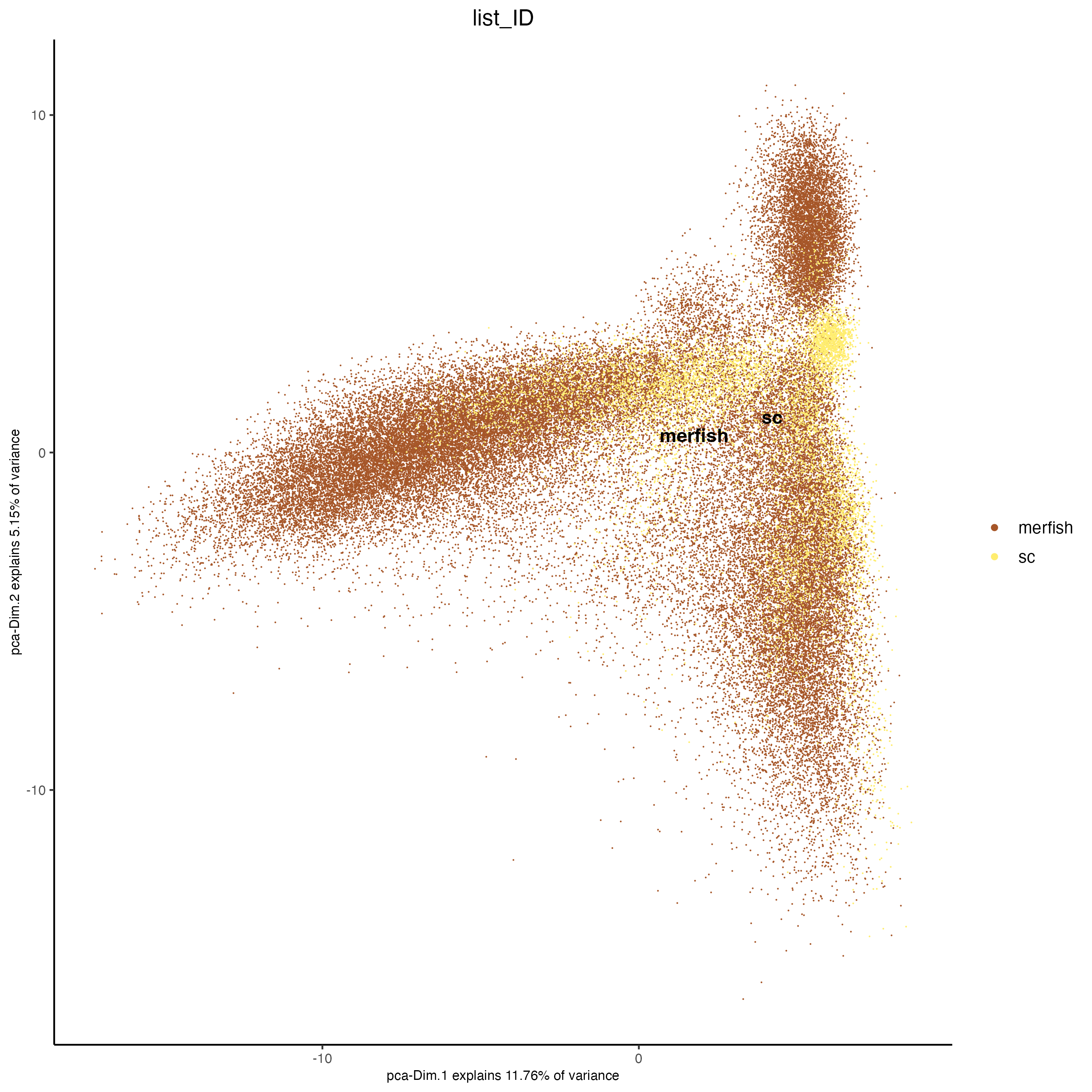
screePlot(j,
          ncp = 50)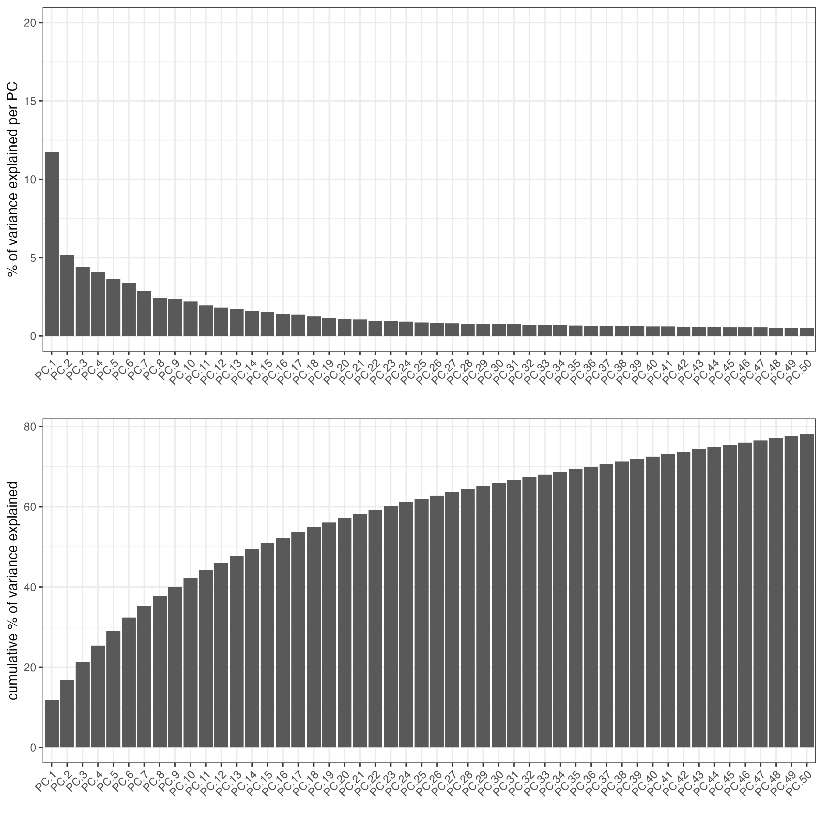
j <- runUMAP(j,
             dimensions_to_use = 1:10)

plotUMAP(j,
         cell_color = "list_ID",
         point_size = 0.5,
         point_border_stroke = 0,
         cell_color_code = c("red", "blue"))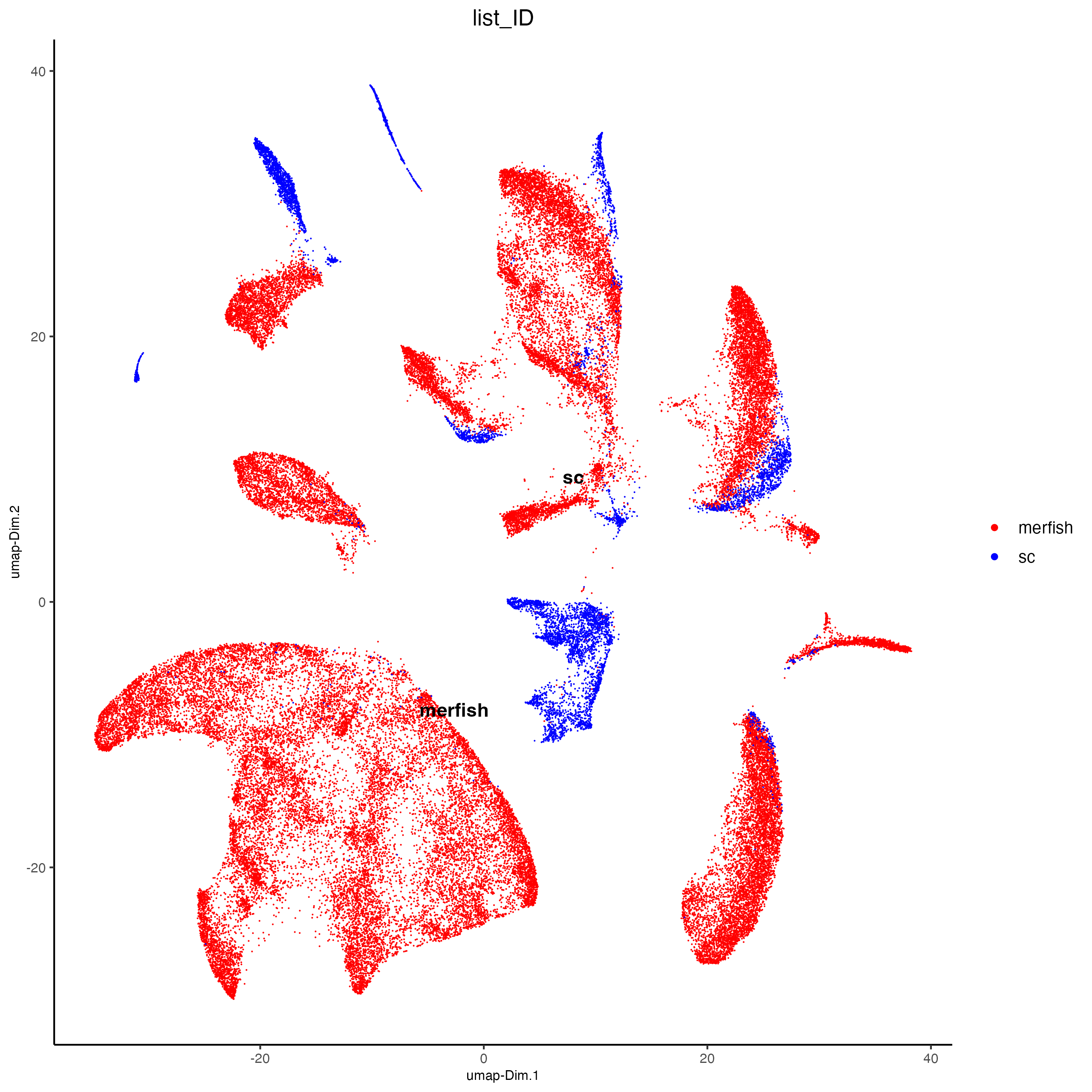
18.5 Process Joined Object (With Harmony Integration)
Run Harmony integration on the PCA space with the “list_ID” (dataset source) as the variable to remove to produce an aligned PCA space that better represents the biology of the datasets.
j <- runGiottoHarmony(j,
                      vars_use = "list_ID",
                      dim_reduction_name = "pca",
                      dimensions_to_use = 1:10,
                      name = "harmony")

j <- runUMAP(j,
             dim_reduction_to_use = "harmony",
             dim_reduction_name = "harmony",
             name = "umap_harmony",
             dimensions_to_use = 1:10)

plotUMAP(j,
         cell_color = "Class",
         dim_reduction_name = "umap_harmony",
         point_size = 0.5,
         select_cells = spatIDs(j, subset = list_ID == "sc"),
         point_border_stroke = 0,
         other_point_size = 0.3)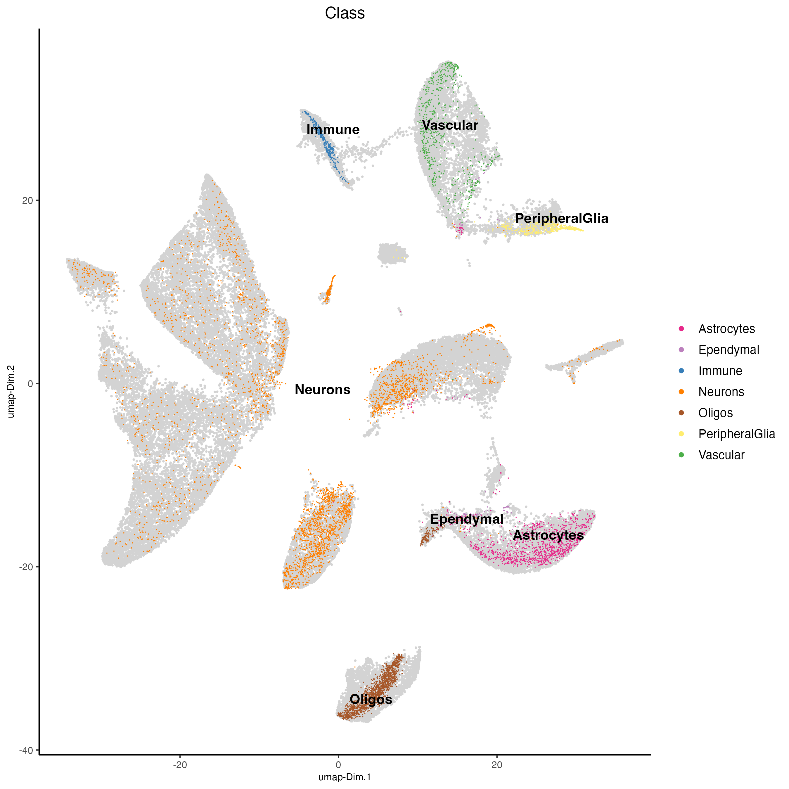
18.6 Label transferring
The single-cell-based cell-type annotations map to the clustering of the integrated dataset. We can now transfer these annotations using labelTransfer() from just the single cells (source_cell_ids) to the rest of the cells (merfish data cells) using kNN clustering.
j <- labelTransfer(j,
                   source_cell_ids = spatIDs(j, subset = list_ID == "sc"),
                   k = 10,
                   labels = "Class",
                   reduction_method = "harmony",
                   reduction_name = "harmony",
                   dimensions_to_use = 1:10)

plotUMAP(j,
         cell_color = "trnsfr_Class",
         dim_reduction_name = "umap_harmony",
         point_size = 0.5,
         point_border_stroke = 0)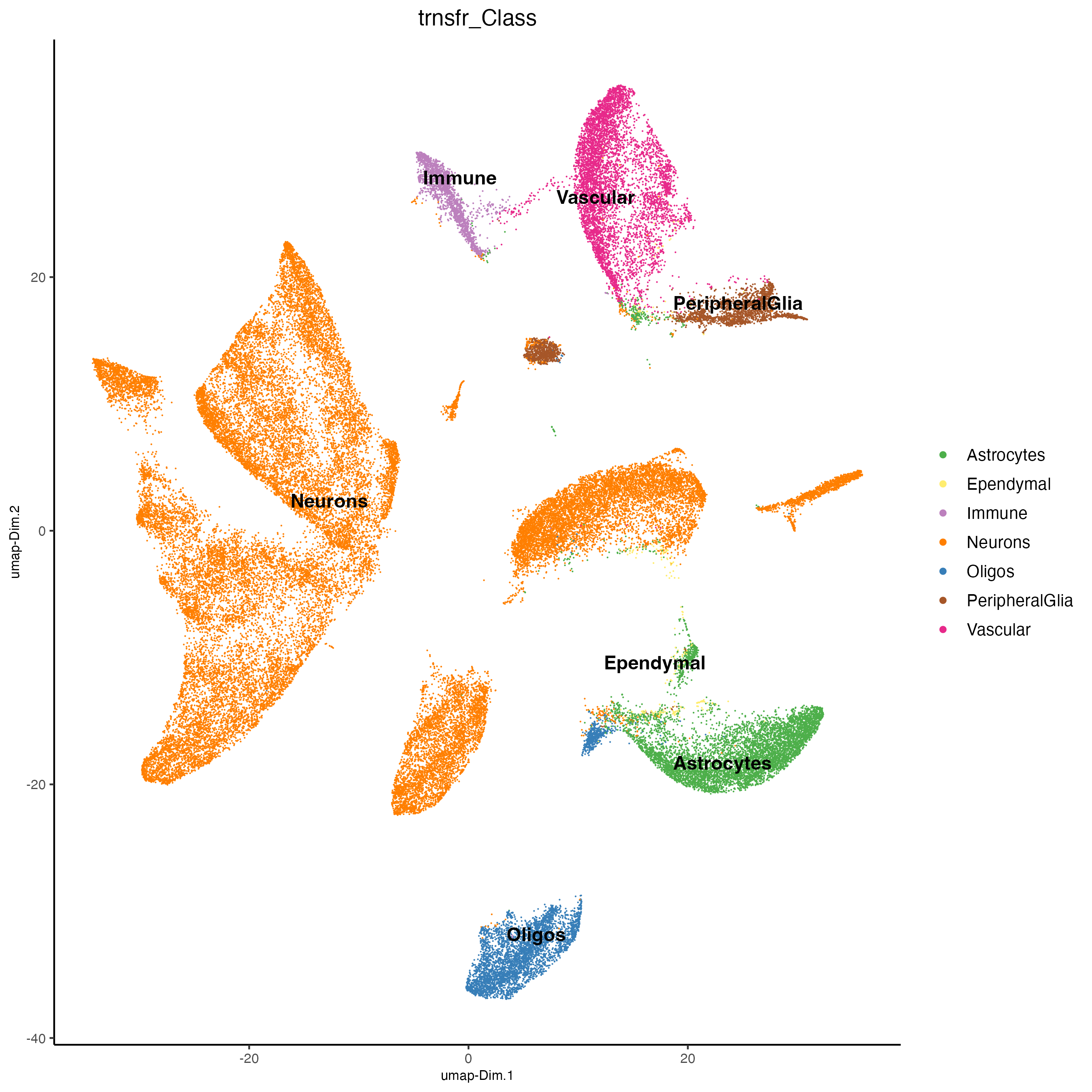
18.7 Add transferred labels to the original merfish object
j_cellmetadata <- pDataDT(j)
j_cellmetadata <- j_cellmetadata[list_ID == "merfish",]
j_cellmetadata[, cell_ID := gsub("^merfish-", "", cell_ID)]
j_cellmetadata <- j_cellmetadata[, .(cell_ID, trnsfr_Class, trnsfr_Class_prob)]

g_s1 <- addCellMetadata(g_s1,
                        new_metadata = j_cellmetadata,
                        by_column = TRUE,
                        column_cell_ID = "cell_ID")

spatPlot2D(g_s1,
           cell_color = "trnsfr_Class",
           point_size = 1)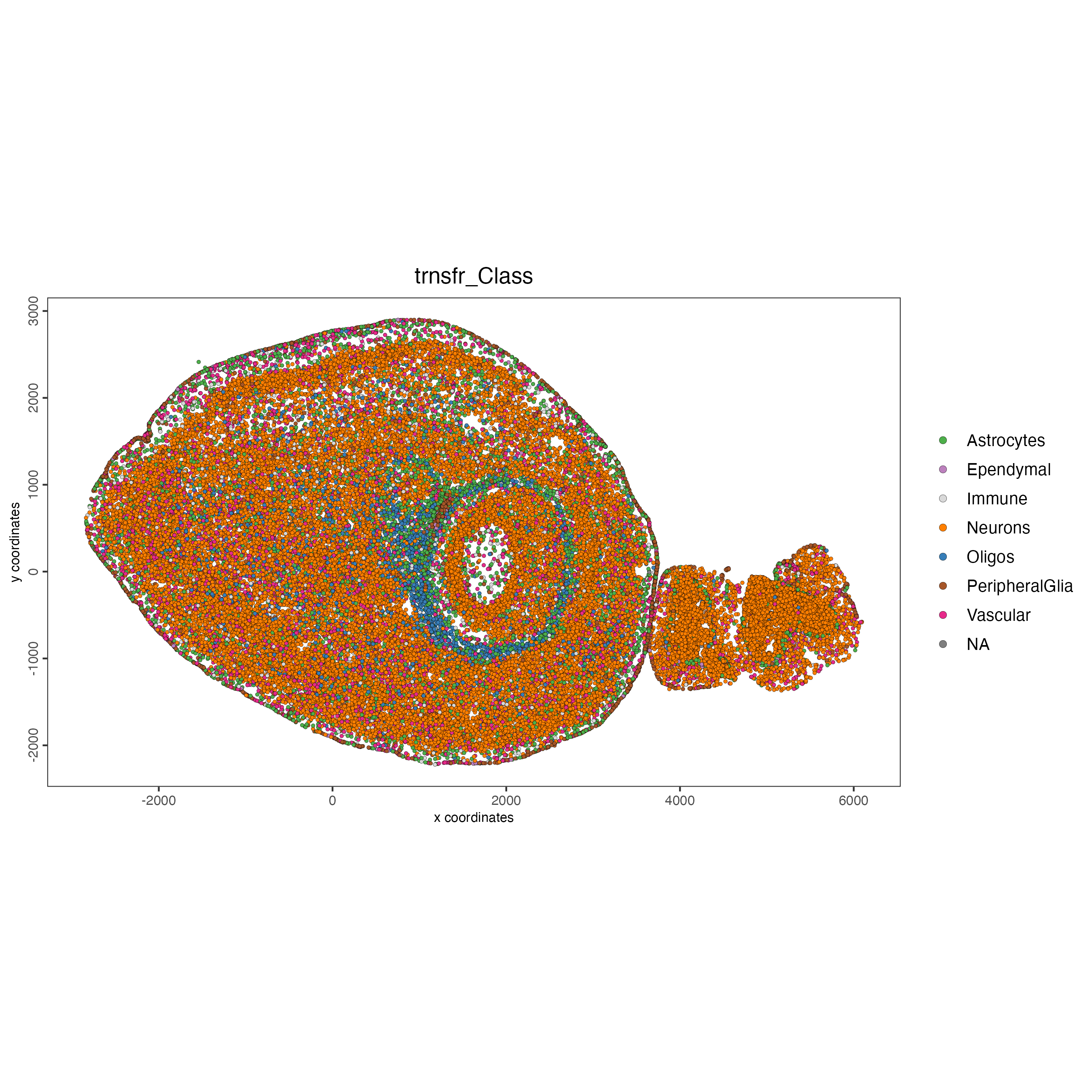
19 Session info
R version 4.5.0 (2025-04-11)
Platform: x86_64-apple-darwin20
Running under: macOS Sequoia 15.4.1

Matrix products: default
BLAS:   /System/Library/Frameworks/Accelerate.framework/Versions/A/Frameworks/vecLib.framework/Versions/A/libBLAS.dylib
LAPACK: /Library/Frameworks/R.framework/Versions/4.5-x86_64/Resources/lib/libRlapack.dylib;  LAPACK version 3.12.1

locale:
[1] en_US.UTF-8/en_US.UTF-8/en_US.UTF-8/C/en_US.UTF-8/en_US.UTF-8

time zone: America/New_York
tzcode source: internal

attached base packages:
[1] stats     graphics  grDevices utils     datasets  methods   base

other attached packages:
[1] Giotto_4.2.1      GiottoClass_0.4.7

loaded via a namespace (and not attached):
  [1] RColorBrewer_1.1-3          rstudioapi_0.17.1           jsonlite_2.0.0
  [4] magrittr_2.0.3              farver_2.1.2                rmarkdown_2.29
  [7] ragg_1.4.0                  vctrs_0.6.5                 memoise_2.0.1
 [10] GiottoUtils_0.2.4           terra_1.8-50                htmltools_0.5.8.1
 [13] S4Arrays_1.8.0              curl_6.2.2                  BiocNeighbors_2.2.0
 [16] SparseArray_1.8.0           htmlwidgets_1.6.4           desc_1.4.3
 [19] plotly_4.10.4               cachem_1.1.0                igraph_2.1.4
 [22] lifecycle_1.0.4             pkgconfig_2.0.3             rsvd_1.0.5
 [25] Matrix_1.7-3                R6_2.6.1                    fastmap_1.2.0
 [28] GenomeInfoDbData_1.2.14     MatrixGenerics_1.20.0       digest_0.6.37
 [31] colorspace_2.1-1            S4Vectors_0.46.0            ps_1.9.1
 [34] dqrng_0.4.1                 irlba_2.3.5.1               textshaping_1.0.1
 [37] GenomicRanges_1.60.0        beachmat_2.24.0             labeling_0.4.3
 [40] progressr_0.15.1            httr_1.4.7                  polyclip_1.10-7
 [43] abind_1.4-8                 compiler_4.5.0              remotes_2.5.0
 [46] withr_3.0.2                 backports_1.5.0             BiocParallel_1.42.0
 [49] viridis_0.6.5               pkgbuild_1.4.7              ggforce_0.4.2
 [52] R.utils_2.13.0              MASS_7.3-65                 DelayedArray_0.34.1
 [55] bluster_1.18.0              gtools_3.9.5                GiottoVisuals_0.2.12
 [58] tools_4.5.0                 R.oo_1.27.1                 glue_1.8.0
 [61] dbscan_1.2.2                callr_3.7.6                 grid_4.5.0
 [64] checkmate_2.3.2             Rtsne_0.17                  cluster_2.1.8.1
 [67] generics_0.1.4              gtable_0.3.6                R.methodsS3_1.8.2
 [70] tidyr_1.3.1                 data.table_1.17.2           BiocSingular_1.24.0
 [73] tidygraph_1.3.1             ScaledMatrix_1.16.0         metapod_1.16.0
 [76] XVector_0.48.0              BiocGenerics_0.54.0         RcppAnnoy_0.0.22
 [79] ggrepel_0.9.6               pillar_1.10.2               limma_3.64.0
 [82] dplyr_1.1.4                 tweenr_2.0.3                lattice_0.22-7
 [85] FNN_1.1.4.1                 tidyselect_1.2.1            SingleCellExperiment_1.30.1
 [88] locfit_1.5-9.12             scuttle_1.18.0              knitr_1.50
 [91] gridExtra_2.3               IRanges_2.42.0              edgeR_4.6.2
 [94] SummarizedExperiment_1.38.1 scattermore_1.2             RhpcBLASctl_0.23-42
 [97] stats4_4.5.0                xfun_0.52                   graphlayouts_1.2.2
[100] Biobase_2.68.0              statmod_1.5.0               matrixStats_1.5.0
[103] UCSC.utils_1.4.0            lazyeval_0.2.2              yaml_2.3.10
[106] evaluate_1.0.3              codetools_0.2-20            ggraph_2.2.1
[109] GiottoData_0.2.16           tibble_3.2.1                BiocManager_1.30.25
[112] colorRamp2_0.1.0            cli_3.6.5                   uwot_0.2.3
[115] reticulate_1.42.0           systemfonts_1.2.3           processx_3.8.6
[118] harmony_1.2.3               Rcpp_1.0.14                 GenomeInfoDb_1.44.0
[121] png_0.1-8                   parallel_4.5.0              ggplot2_3.5.2
[124] scran_1.36.0                viridisLite_0.4.2           scales_1.4.0
[127] purrr_1.0.4                 crayon_1.5.3                rlang_1.1.6
[130] cowplot_1.1.3