Analyzing NeMO Slide-seq datasets on Terra bio
Source:vignettes/nemo_slideseq.Rmd
nemo_slideseq.Rmd1 Identify the NeMO dataset
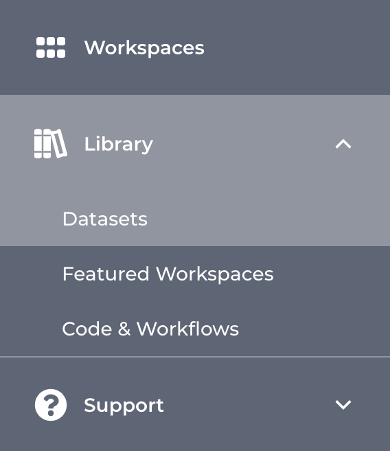
Log in to your Terra bio account and go to the left menu, select Library > Datasets
On the datasets page, scroll down until you find the NeMO database
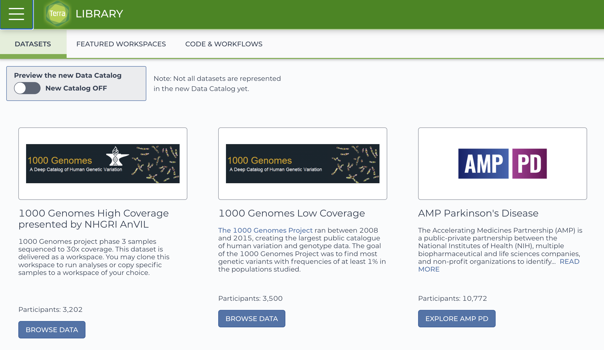

2 Load the dataset to a terra workspace
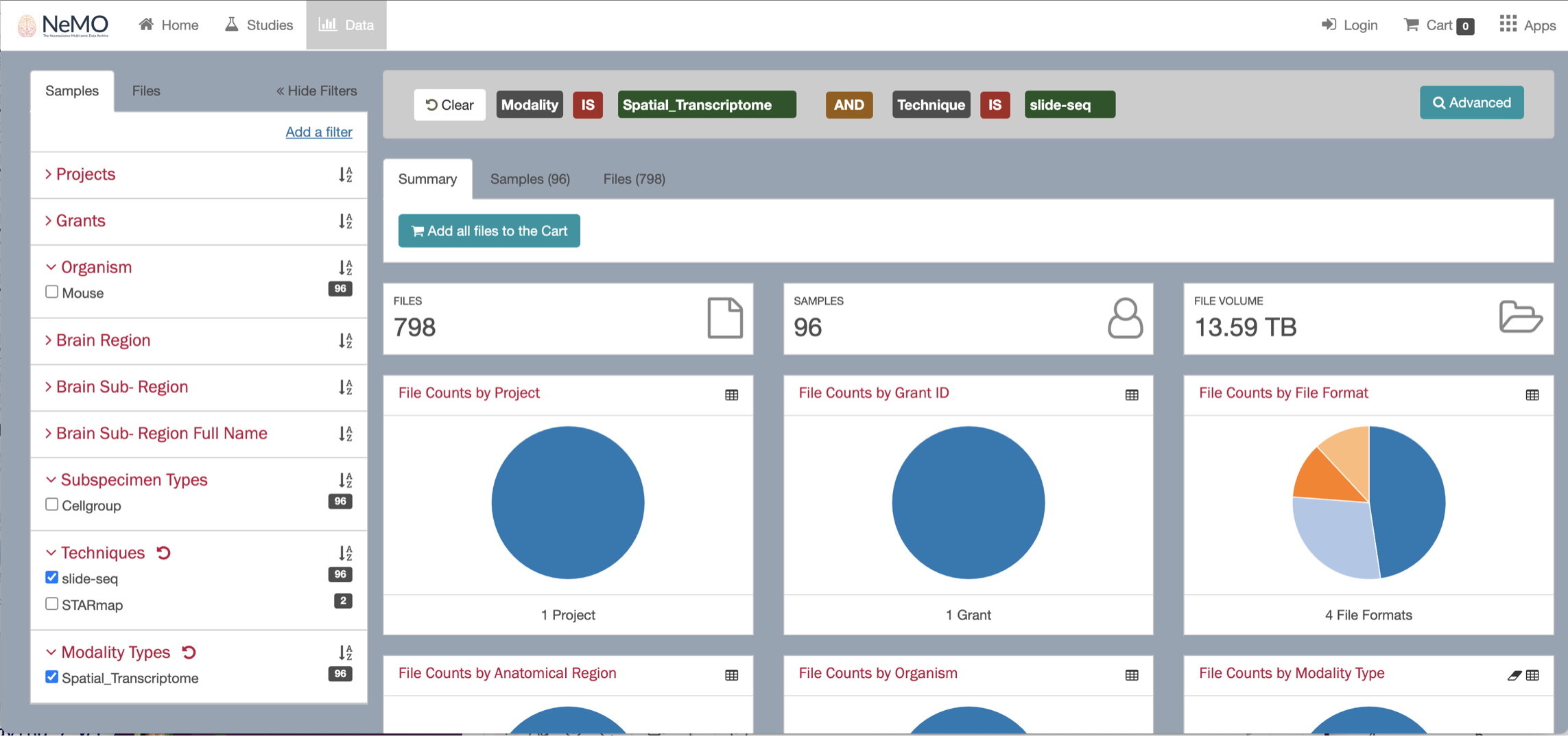
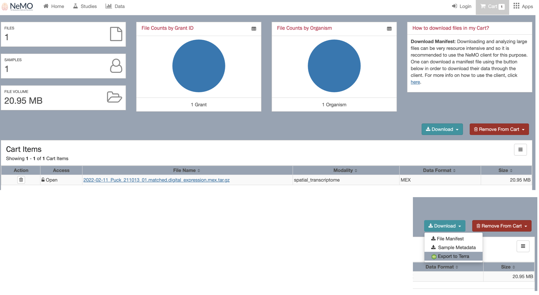
By clicking on the Browse data button, you will be re-directed to the NeMO website. Use the filters menu to select the Slide-seq technology, then chose a sample to download and ddd the file to the cart.
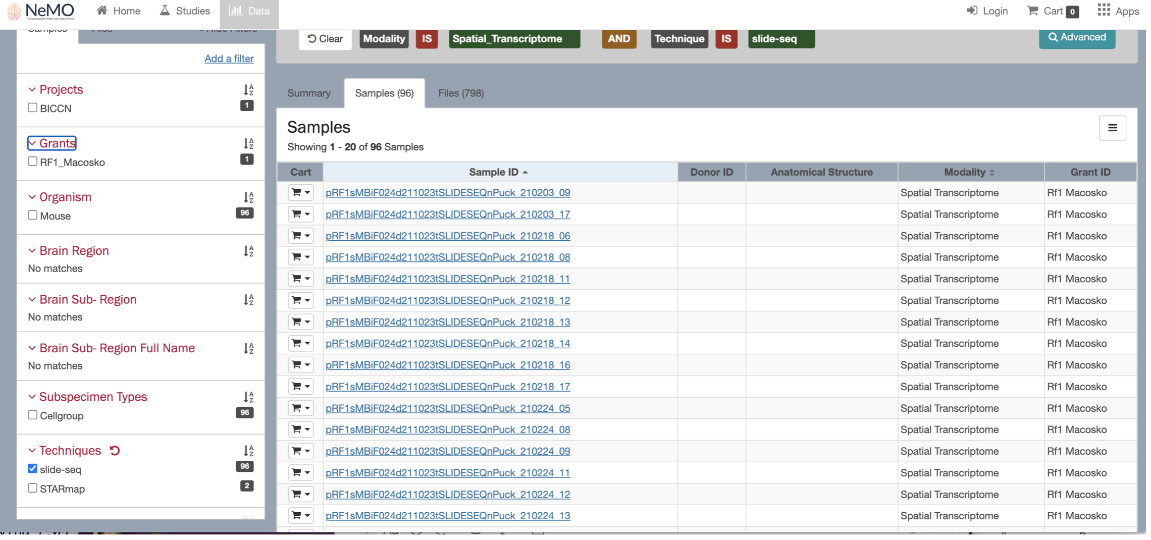
When selecting the sample, you will see multiple files available to download, including the fasta files. Uncheck the fasta files boxes and keep only the expression.mex.tar.gz file.
Click the Download button and select the option “Export to terra”.
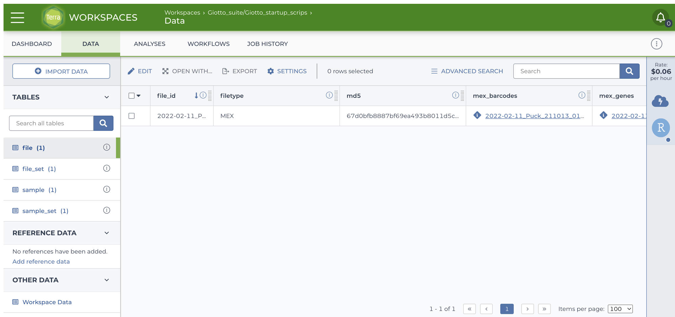
You will be directed back to your terra bio account. Select the Workspace to add your dataset.
You will find the new file under the Data tab > file section.
3 Open the dataset
Scroll to the right and locate the url of the file, it should look like https://data.nemoarchive.org/biccn/grant/rf1_macosko/macosko/spatial_transcriptome/cellgroup/Slide-seq/mouse/processed/counts/2022-02-11_Puck_211013_01.matched.digital_expression.mex.tar.gz.
Open an cloud environment, either using Jupyter notebooks or RStudio.
Open the terminal and load the file to your session by running the
command wget <file url>. Uncompress the file, you
will get a folder with three files:
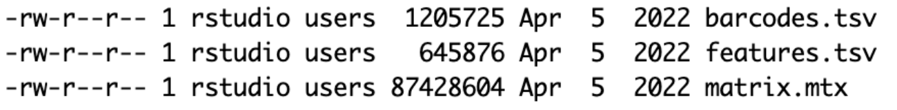
Use these files to create a Giotto object and start running the analysis.
4 Run the analysis
You can use the following Giotto pipeline as an example. The sample 2020-12-19_Puck_201112_26 was used for running this tutorial.
4.1 Download the data to your R session
- Get the expression data
download.file(url = "https://data.nemoarchive.org/biccn/grant/rf1_macosko/macosko/spatial_transcriptome/cellgroup/Slide-seq/mouse/processed/counts/2020-12-19_Puck_201112_26.matched.digital_expression.mex.tar.gz",
destfile = file.path(data_path, "2020-12-19_Puck_201112_26.matched.digital_expression.mex.tar.gz"))- Get the spatial coordinates
download.file(url = "https://data.nemoarchive.org/biccn/grant/rf1_macosko/macosko/spatial_transcriptome/cellgroup/Slide-seq/mouse/processed/other/2020-12-19_Puck_201112_26.BeadLocationsForR.csv.tar",
destfile = file.path(data_path, "2020-12-19_Puck_201112_26.BeadLocationsForR.csv.tar"))- Untar the expression files running:
4.2 Load the package and set instructions
library(Giotto)

# 1. set results directory
results_folder <- "/path/to/results/"

# 2. set giotto python path
# set python path to your preferred python version path
# set python path to NULL if you want to automatically install (only the 1st time) and use the giotto miniconda environment
python_path <- NULL

# 3. create giotto instructions
instructions <- createGiottoInstructions(save_dir = results_folder,
                                         save_plot = TRUE,
                                         show_plot = FALSE,
                                         return_plot = FALSE,
                                         python_path = python_path)
4.3 Create Giotto object
- Read the expression files and create the expression matrix.
expression_matrix <- get10Xmatrix("2020-12-19_Puck_201112_26.matched.digital_expression")- Read the spatial coordinates file and filter the cell IDs.
spatial_locs <- data.table::fread("2020-12-19_Puck_201112_26.BeadLocationsForR.csv.tar")

spatial_locs <- spatial_locs[spatial_locs$barcodes %in% colnames(expression_matrix),]- Create the Giotto object
giotto_object <- createGiottoObject(
  expression = expression_matrix,
  spatial_locs = spatial_locs,
  instructions = instructions
)- Visualize the dataset
spatPlot2D(giotto_object,
           point_size = 2)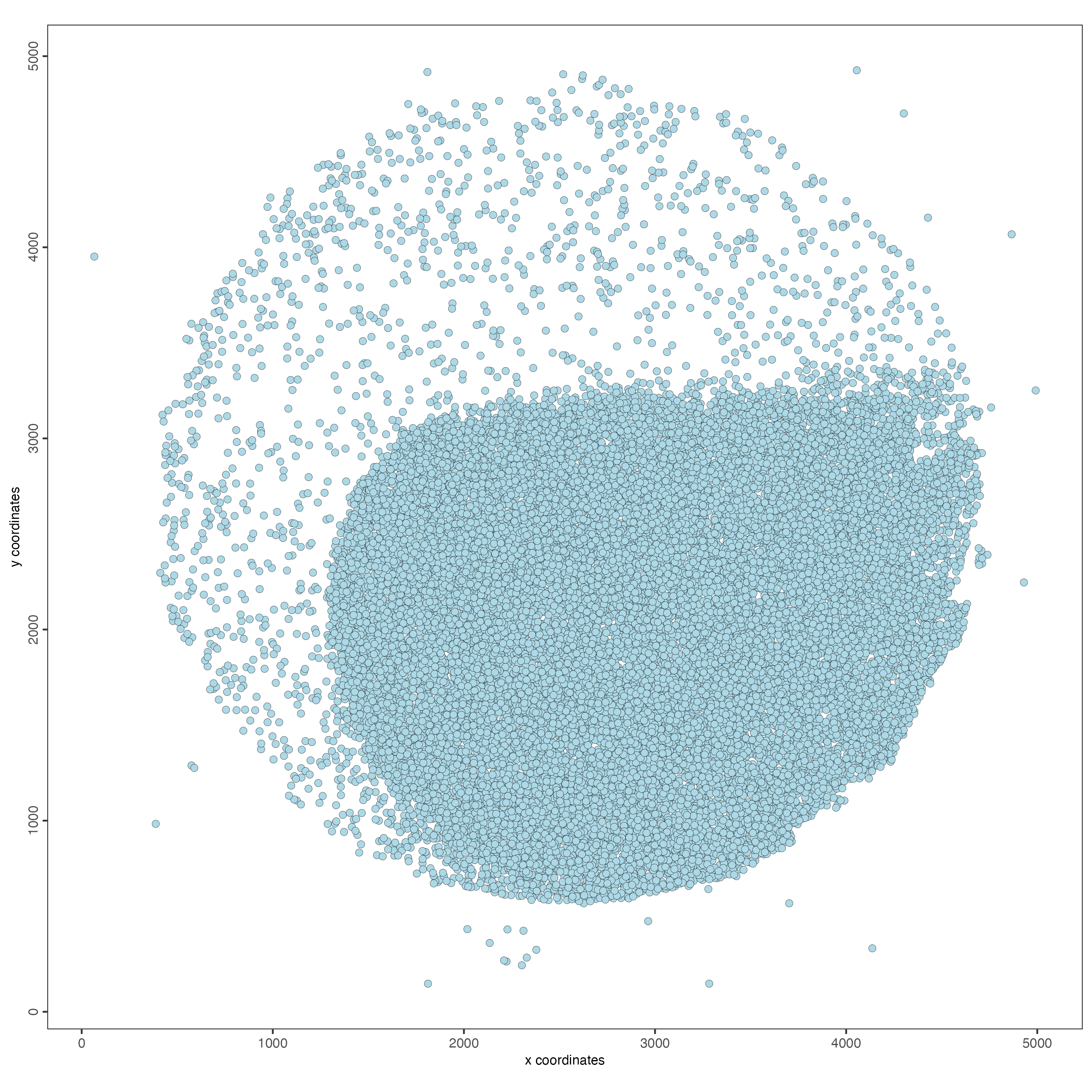
4.4 Filtering
giotto_object <- filterGiotto(giotto_object,
                              min_det_feats_per_cell = 10,
                              feat_det_in_min_cells = 10)
4.5 Normalization
giotto_object <- normalizeGiotto(giotto_object)4.6 Add statistics
giotto_object <- addStatistics(giotto_object)

spatPlot2D(giotto_object,
           cell_color = "nr_feats",
           color_as_factor = FALSE,
           point_size = 1)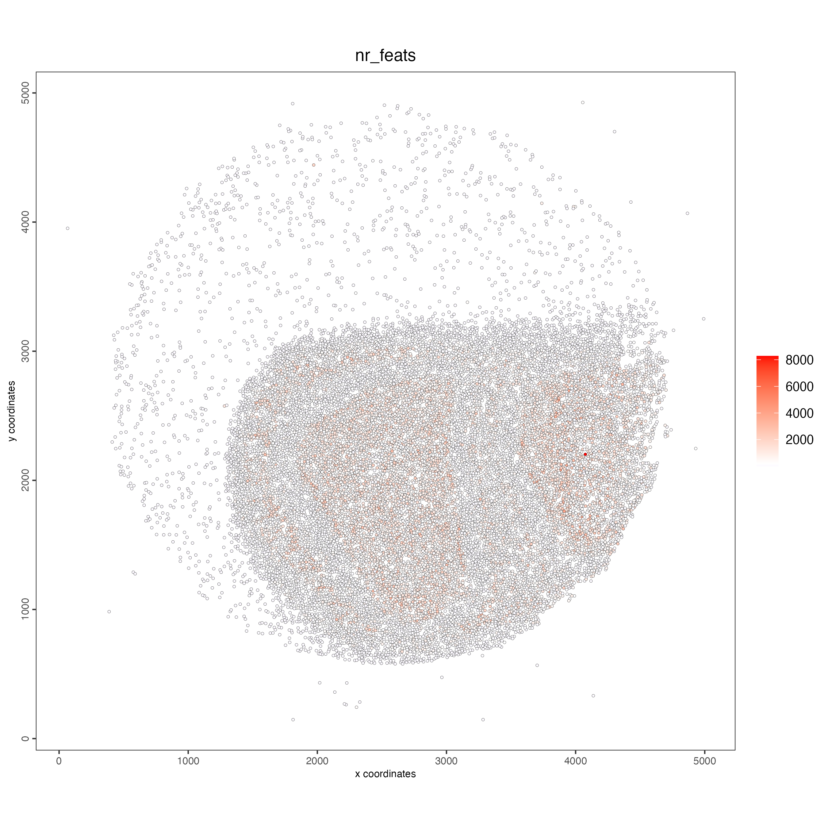
4.8 Clustering
giotto_object <- runUMAP(giotto_object,
                         dimensions_to_use = 1:10)

giotto_object <- createNearestNetwork(giotto_object)

giotto_object <- doLeidenCluster(giotto_object,
                                 resolution = 1)
4.9 Plot
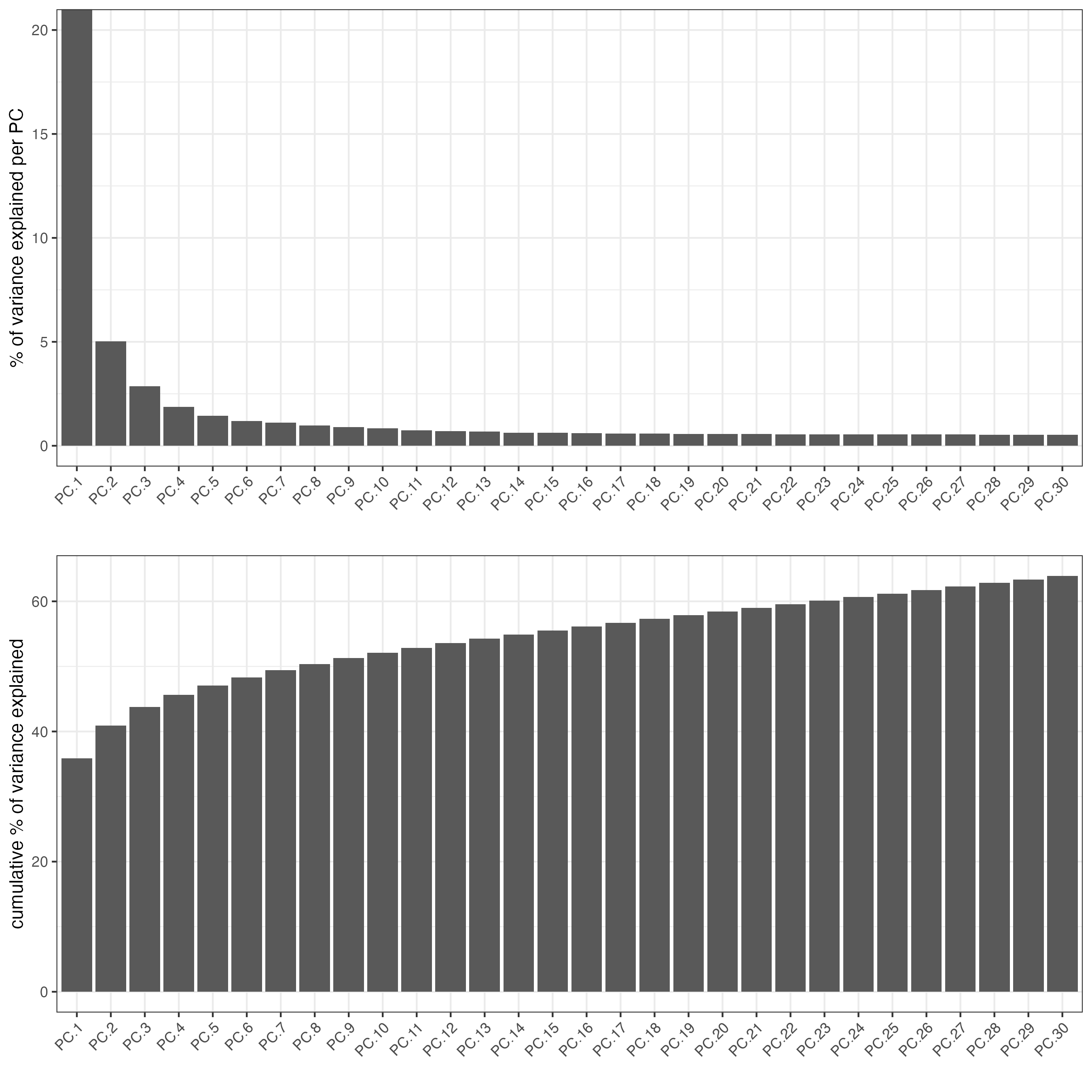
plotPCA(giotto_object,
        cell_color = "leiden_clus",
        point_size = 1)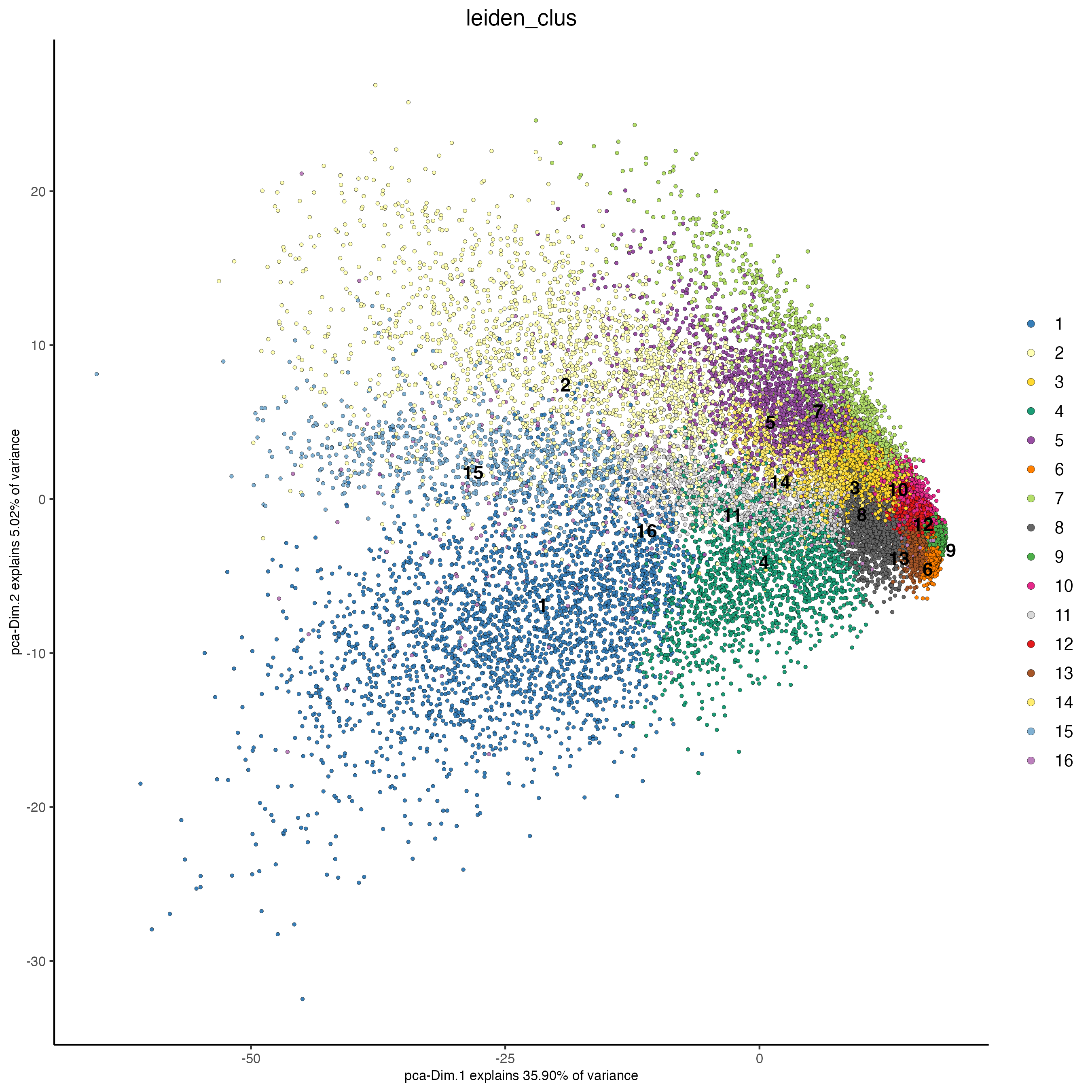
plotUMAP(giotto_object,
         cell_color = "leiden_clus",
         point_size = 1)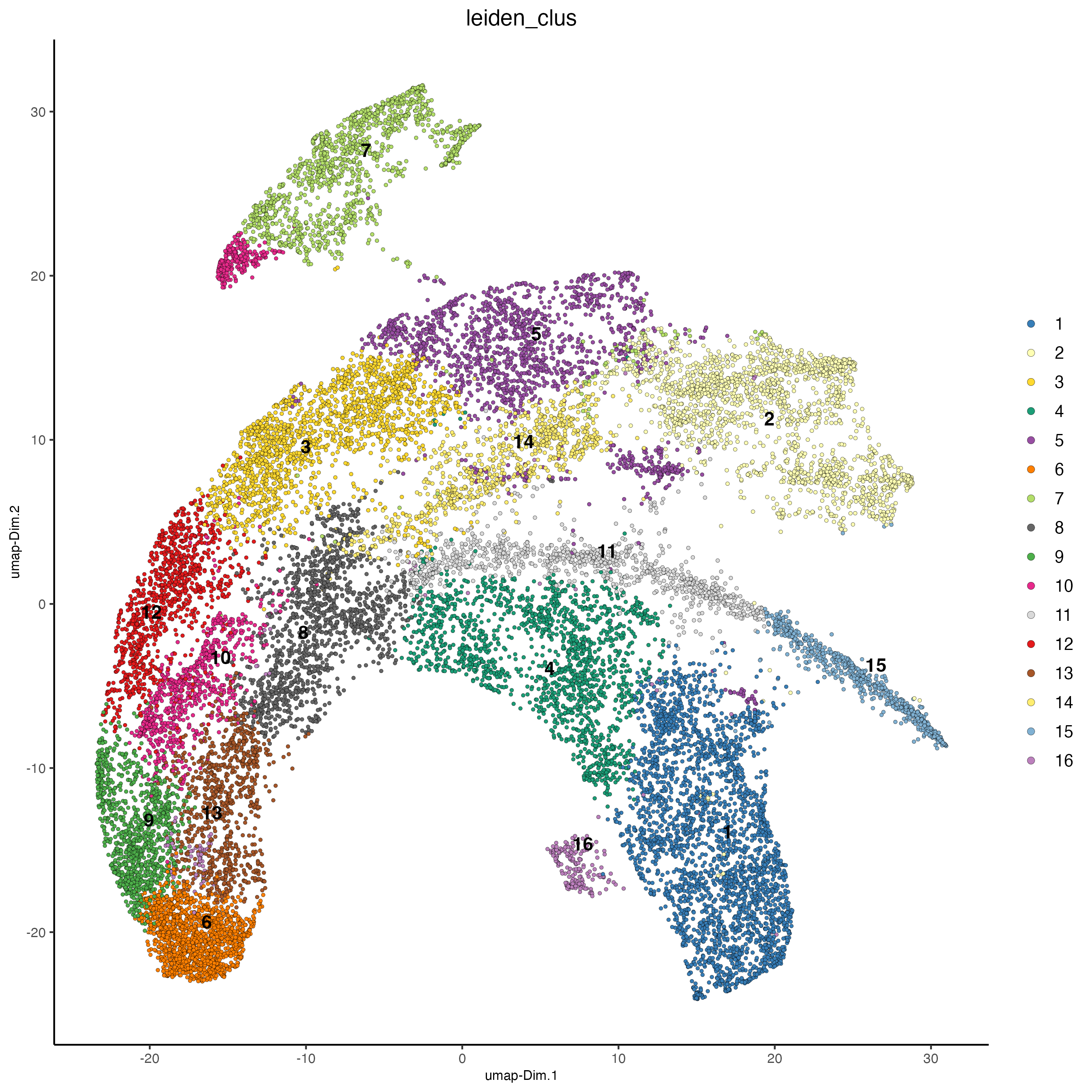
spatPlot2D(giotto_object,
           cell_color = "leiden_clus",
           point_size = 1)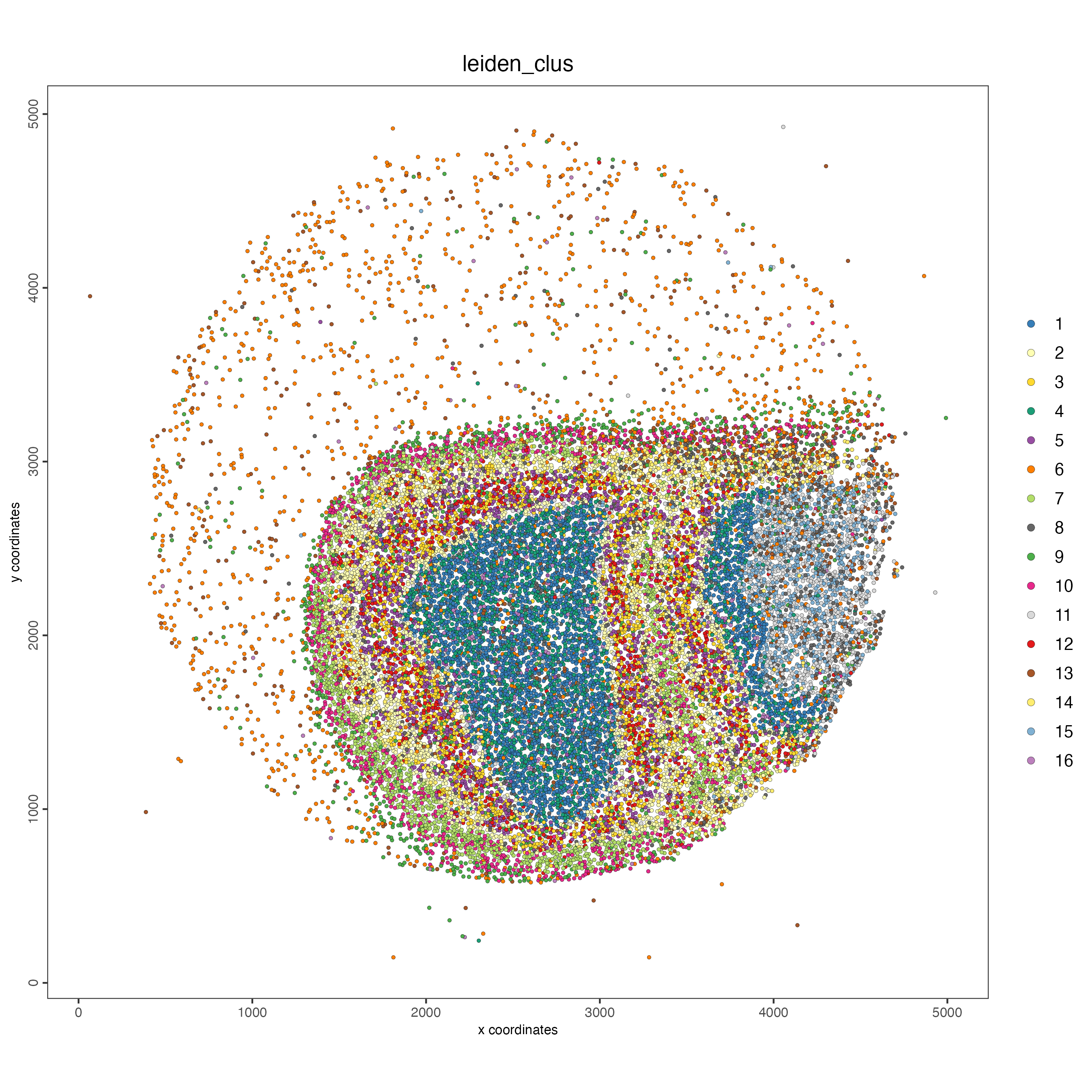
5 Session info
R version 4.4.0 (2024-04-24)
Platform: x86_64-apple-darwin20
Running under: macOS Sonoma 14.6.1

Matrix products: default
BLAS:   /System/Library/Frameworks/Accelerate.framework/Versions/A/Frameworks/vecLib.framework/Versions/A/libBLAS.dylib
LAPACK: /Library/Frameworks/R.framework/Versions/4.4-x86_64/Resources/lib/libRlapack.dylib;  LAPACK version 3.12.0

locale:
[1] en_US.UTF-8/en_US.UTF-8/en_US.UTF-8/C/en_US.UTF-8/en_US.UTF-8

time zone: America/New_York
tzcode source: internal

attached base packages:
[1] stats     graphics  grDevices utils     datasets  methods   base

other attached packages:
[1] Giotto_4.1.1      GiottoClass_0.3.5

loaded via a namespace (and not attached):
  [1] colorRamp2_0.1.0            deldir_2.0-4
  [3] rlang_1.1.4                 magrittr_2.0.3
  [5] RcppAnnoy_0.0.22            GiottoUtils_0.1.11
  [7] matrixStats_1.3.0           compiler_4.4.0
  [9] png_0.1-8                   systemfonts_1.1.0
 [11] vctrs_0.6.5                 reshape2_1.4.4
 [13] stringr_1.5.1               pkgconfig_2.0.3
 [15] SpatialExperiment_1.14.0    crayon_1.5.3
 [17] fastmap_1.2.0               backports_1.5.0
 [19] magick_2.8.4                XVector_0.44.0
 [21] labeling_0.4.3              utf8_1.2.4
 [23] rmarkdown_2.28              UCSC.utils_1.0.0
 [25] ragg_1.3.2                  purrr_1.0.2
 [27] xfun_0.47                   beachmat_2.20.0
 [29] zlibbioc_1.50.0             GenomeInfoDb_1.40.1
 [31] jsonlite_1.8.8              DelayedArray_0.30.1
 [33] BiocParallel_1.38.0         terra_1.7-78
 [35] irlba_2.3.5.1               parallel_4.4.0
 [37] R6_2.5.1                    stringi_1.8.4
 [39] RColorBrewer_1.1-3          reticulate_1.38.0
 [41] GenomicRanges_1.56.1        scattermore_1.2
 [43] Rcpp_1.0.13                 SummarizedExperiment_1.34.0
 [45] knitr_1.48                  R.utils_2.12.3
 [47] IRanges_2.38.1              Matrix_1.7-0
 [49] igraph_2.0.3                tidyselect_1.2.1
 [51] rstudioapi_0.16.0           abind_1.4-5
 [53] yaml_2.3.10                 codetools_0.2-20
 [55] lattice_0.22-6              tibble_3.2.1
 [57] plyr_1.8.9                  Biobase_2.64.0
 [59] withr_3.0.1                 evaluate_0.24.0
 [61] pillar_1.9.0                MatrixGenerics_1.16.0
 [63] checkmate_2.3.2             stats4_4.4.0
 [65] plotly_4.10.4               generics_0.1.3
 [67] dbscan_1.2-0                sp_2.1-4
 [69] S4Vectors_0.42.1            ggplot2_3.5.1
 [71] munsell_0.5.1               scales_1.3.0
 [73] gtools_3.9.5                glue_1.7.0
 [75] lazyeval_0.2.2              tools_4.4.0
 [77] GiottoVisuals_0.2.5         data.table_1.15.4
 [79] ScaledMatrix_1.12.0         cowplot_1.1.3
 [81] grid_4.4.0                  tidyr_1.3.1
 [83] colorspace_2.1-1            SingleCellExperiment_1.26.0
 [85] GenomeInfoDbData_1.2.12     BiocSingular_1.20.0
 [87] rsvd_1.0.5                  cli_3.6.3
 [89] textshaping_0.4.0           fansi_1.0.6
 [91] S4Arrays_1.4.1              viridisLite_0.4.2
 [93] dplyr_1.1.4                 uwot_0.2.2
 [95] gtable_0.3.5                R.methodsS3_1.8.2
 [97] digest_0.6.37               BiocGenerics_0.50.0
 [99] SparseArray_1.4.8           ggrepel_0.9.5
[101] rjson_0.2.22                htmlwidgets_1.6.4
[103] farver_2.1.2                htmltools_0.5.8.1
[105] R.oo_1.26.0                 lifecycle_1.0.4
[107] httr_1.4.7