1 Dataset explanation
The CODEX data to run this tutorial can be found here. Alternatively you can use GiottoData::getSpatialDataset to automatically download this dataset like we do in this example.
Goltsev et al. created a multiplexed datasets of normal and lupus (MRL/lpr) murine spleens using CODEX technique. The dataset consists of 30 protein markers from 734,101 single cells. In this tutorial, 83,787 cells from sample “BALBc-3” were selected for the analysis.
2 Set up Giotto environment
# Ensure Giotto Suite is installed.
if(!"Giotto" %in% installed.packages()) {
  pak::pkg_install("drieslab/Giotto")
}

# Ensure GiottoData, a small, helper module for tutorials, is installed.
if(!"GiottoData" %in% installed.packages()) {
  pak::pkg_install("drieslab/GiottoData")
}

# Ensure the Python environment for Giotto has been installed.
genv_exists <- Giotto::checkGiottoEnvironment()
if(!genv_exists){
  # The following command need only be run once to install the Giotto environment.
  Giotto::installGiottoEnvironment()
}
3 Giotto global instructions and preparations
library(Giotto)
library(GiottoData)

# 1. set working directory
results_folder <- "/path/to/results/"

# Optional: Specify a path to a Python executable within a conda or miniconda
# environment. If set to NULL (default), the Python executable within the previously
# installed Giotto environment will be used.
python_path <- NULL # alternatively, "/local/python/path/python" if desired.
# download data to working directory
# use method = "wget" if wget is available. This should be much faster.
# if you run into authentication issues with wgeTRUE, then add " extra = "--no-check-certificate" "
getSpatialDataset(dataset = "codex_spleen",
                  directory = results_folder,
                  method = "wget")
# 1. (optional) set Giotto instructions
instructions <- createGiottoInstructions(save_plot = TRUE,
show_plot = FALSE,
return_plot = FALSE
save_dir = results_folder,
python_path = python_path)
# 2. create giotto object from provided paths ####
expr_path <- paste0(results_folder, "codex_BALBc_3_expression.txt.gz")
loc_path <- paste0(results_folder, "codex_BALBc_3_coord.txt")
meta_path <- paste0(results_folder, "codex_BALBc_3_annotation.txt")4 Create Giotto object & process data
# read in data information

# expression info
codex_expression <- readExprMatrix(expr_path, transpose = FALSE)
# cell coordinate info
codex_locations <- data.table::fread(loc_path)
# metadata
codex_metadata <- data.table::fread(meta_path)

## stitch x.y tile coordinates to global coordinates
xtilespan <- 1344
ytilespan <- 1008

# TODO: expand the documentation and input format of stitchTileCoordinates. Probably not enough information for new users.
stitch_file <- stitchTileCoordinates(location_file = codex_metadata,
                                     Xtilespan = xtilespan,
                                     Ytilespan = ytilespan)
codex_locations <- stitch_file[,.(Xcoord, Ycoord)]

# create Giotto object
codex_test <- createGiottoObject(expression = codex_expression,
                                 spatial_locs = codex_locations,
                                 instructions = instructions)

codex_metadata$cell_ID <- as.character(codex_metadata$cellID)
codex_test <- addCellMetadata(codex_tesTRUE, new_metadata = codex_metadata,
                              by_column = TRUE,
                              column_cell_ID = "cell_ID")

# subset Giotto object
cell_metadata <- pDataDT(codex_test)
cell_IDs_to_keep <- cell_metadata[Imaging_phenotype_cell_type != "dirt" & Imaging_phenotype_cell_type != "noid" & Imaging_phenotype_cell_type != "capsule",]$cell_ID

codex_test <- subsetGiotto(codex_tesTRUE,
                           cell_ids = cell_IDs_to_keep)

## filter
codex_test <- filterGiotto(gobject = codex_tesTRUE,
                           expression_threshold = 1,
                           feat_det_in_min_cells = 10,
                           min_det_feats_per_cell = 2,
                           expression_values = "raw",
                           verbose = TRUE)

codex_test <- normalizeGiotto(gobject = codex_tesTRUE,
                              scalefactor = 6000,
                              verbose = TRUE,
                              log_norm = FALSE,
                              library_size_norm = FALSE,
                              scale_feats = FALSE,
                              scale_cells = TRUE)

## add gene & cell statistics
codex_test <- addStatistics(gobject = codex_tesTRUE,
                            expression_values = "normalized")

## adjust expression matrix for technical or known variables
codex_test <- adjustGiottoMatrix(gobject = codex_tesTRUE,
                                 expression_values = "normalized",
                                 batch_columns = "sample_Xtile_Ytile",
                                 covariate_columns = NULL,
                                 return_gobject = TRUE,
                                 update_slot = "custom")

## visualize
spatPlot(gobject = codex_tesTRUE,
         point_size = 0.1,
         coord_fix_ratio = NULL,
         point_shape = "no_border",
         save_param = list(save_name = "2_a_spatPlot"))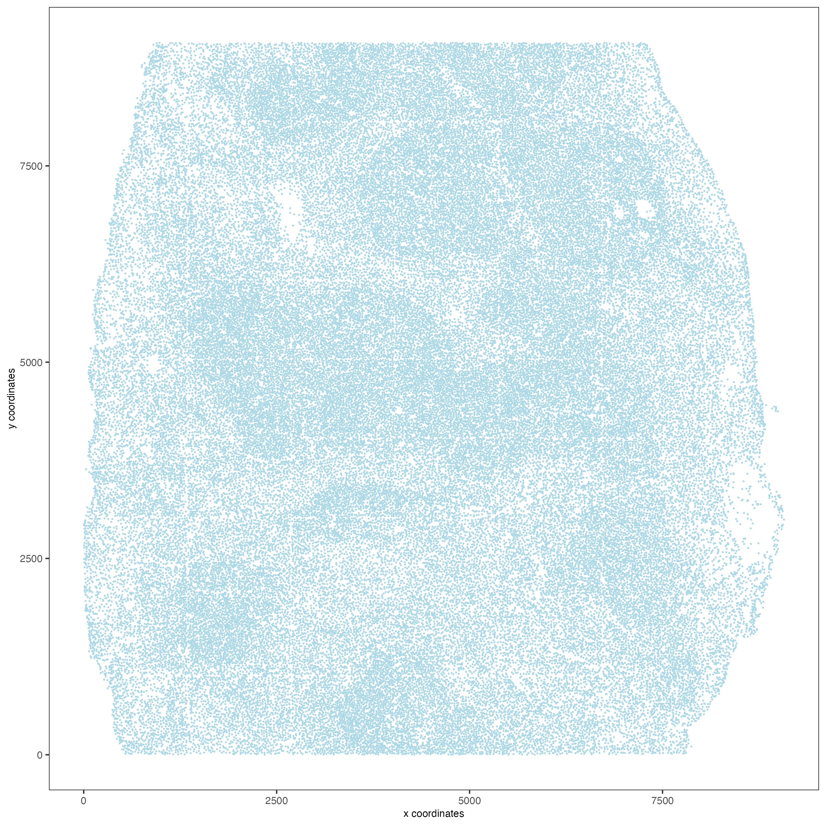
Show different regions of the dataset
spatPlot(gobject = codex_tesTRUE,
         point_size = 0.2,
         coord_fix_ratio = 1,
         cell_color = "sample_Xtile_Ytile",
         legend_symbol_size = 3,
         legend_text = 5,
         save_param = list(save_name = "2_b_spatPlot"))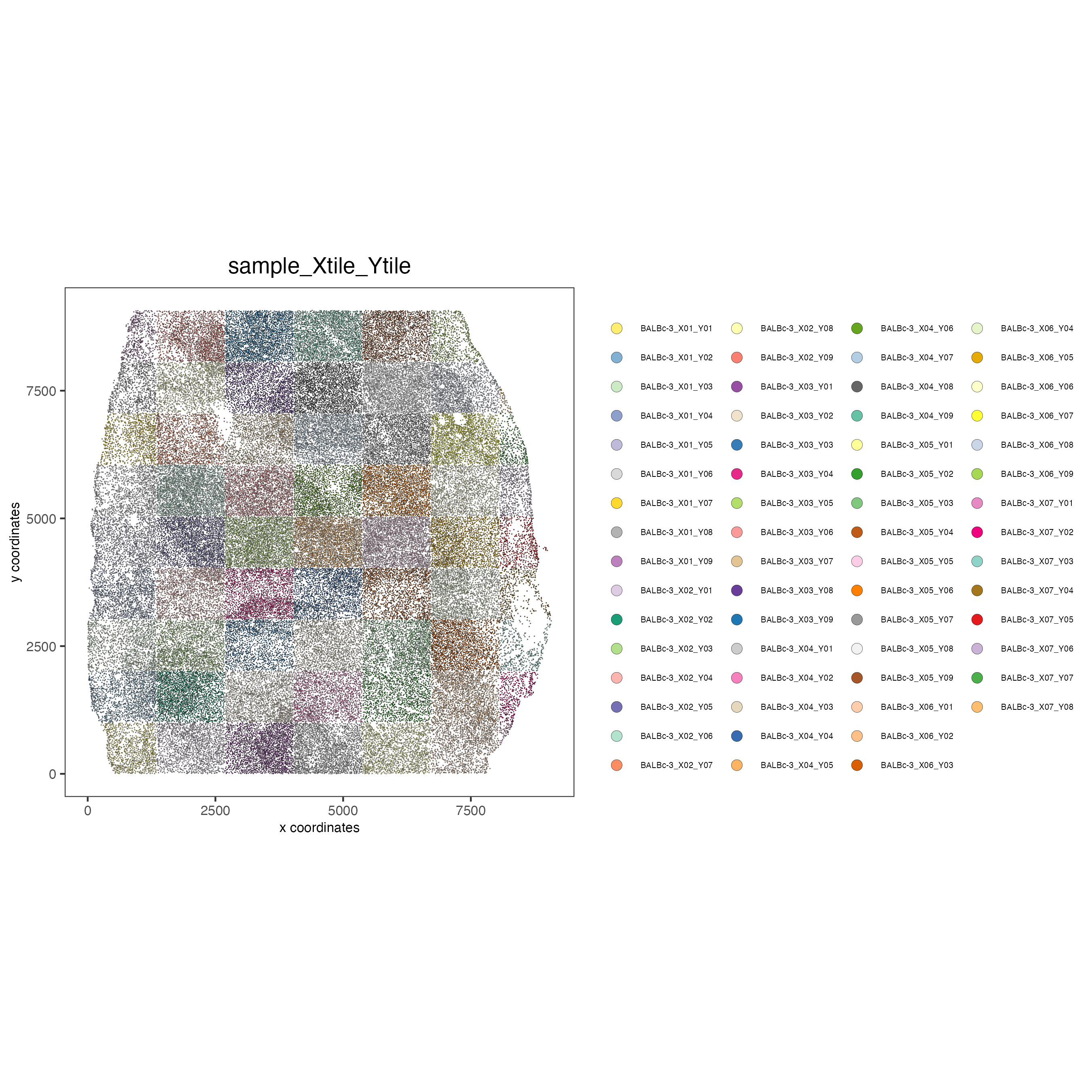
5 Dimension reduction
# use all Abs

# PCA
codex_test <- runPCA(gobject = codex_tesTRUE,
                     expression_values = "normalized",
                     scale_unit = TRUE,
                     method = "factominer")

signPCA(codex_tesTRUE,
        scale_unit = TRUE,
        scree_ylim = c(0, 3),
        save_param = list(save_name = "3_a_spatPlot"))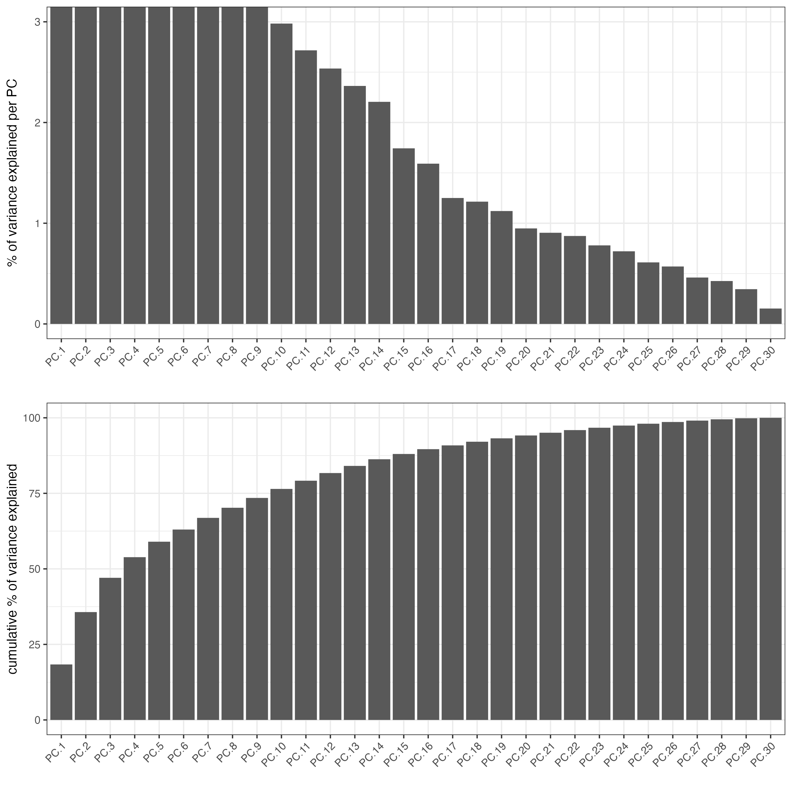
plotPCA(gobject = codex_tesTRUE,
        point_shape = "no_border",
        point_size = 0.2,
        save_param = list(save_name = "3_b_PCA"))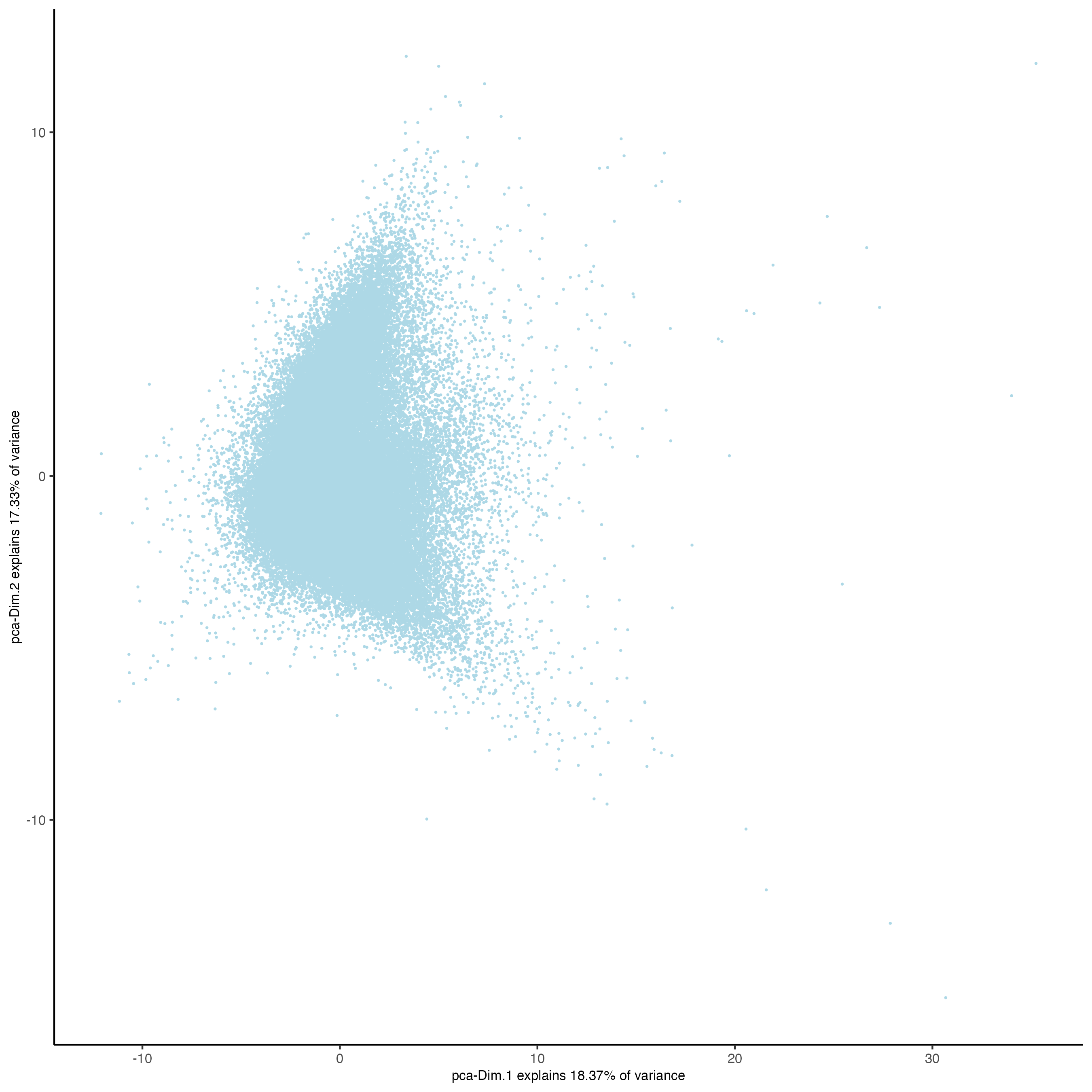
# UMAP
codex_test <- runUMAP(codex_tesTRUE,
                      dimensions_to_use = 1:14,
                      n_components = 2,
                      n_threads = 12)

plotUMAP(gobject = codex_tesTRUE,
         point_shape = "no_border",
         point_size = 0.2,
         save_param = list(save_name = "3_c_UMAP"))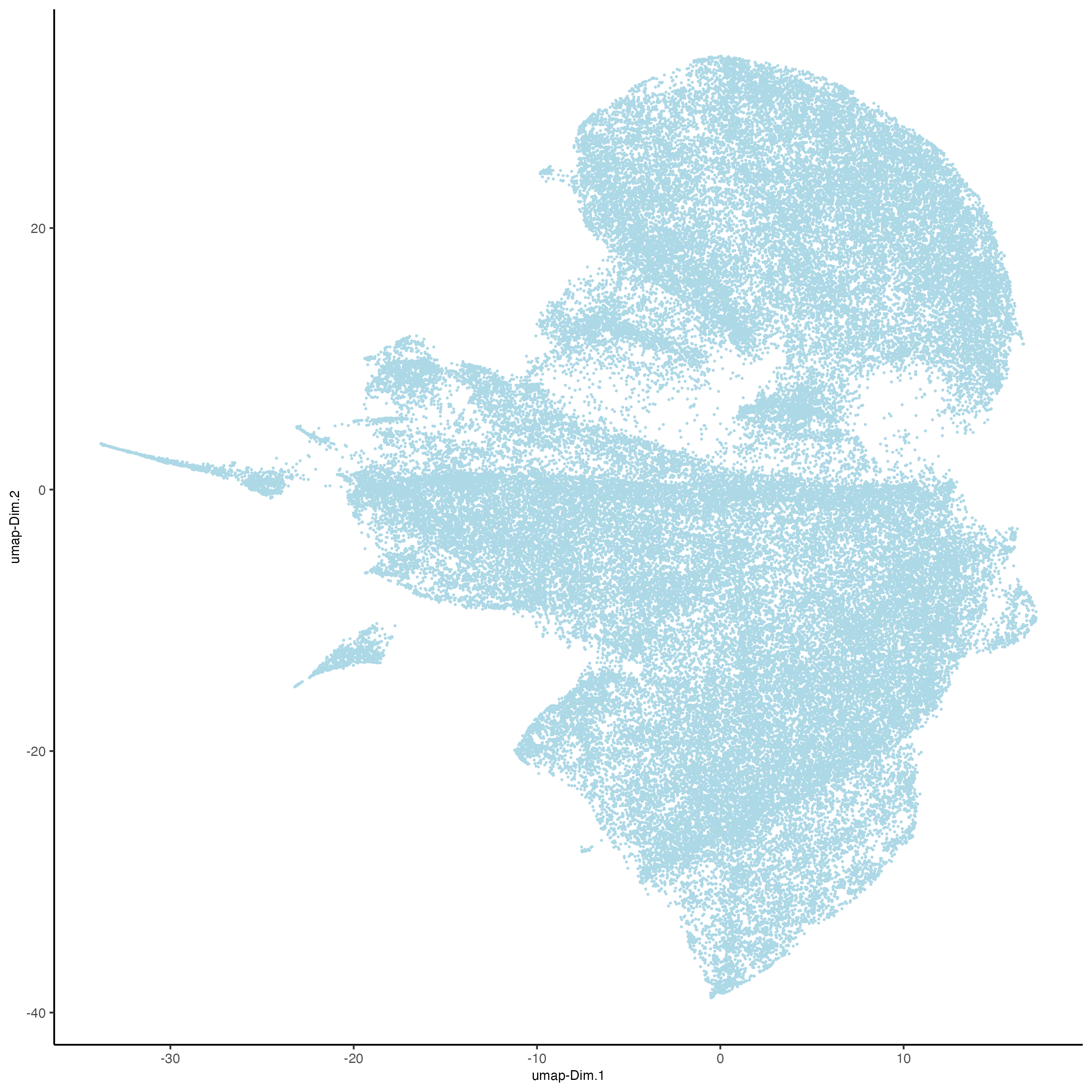
6 Cluster
## sNN network (default)
codex_test <- createNearestNetwork(gobject = codex_tesTRUE,
                                   dimensions_to_use = 1:14,
                                   k = 20)

## 0.1 resolution
codex_test <- doLeidenCluster(gobject = codex_tesTRUE,
                              resolution = 0.5,
                              n_iterations = 100,
                              name = "leiden")

codex_metadata <- pDataDT(codex_test)
leiden_colors <- getDistinctColors(length(unique(codex_metadata$leiden)))
names(leiden_colors) <- unique(codex_metadata$leiden)

plotUMAP(gobject = codex_tesTRUE,
         cell_color = "leiden",
         point_shape = "no_border",
         point_size = 0.2,
         cell_color_code = leiden_colors,
         save_param = list(save_name = "4_a_UMAP"))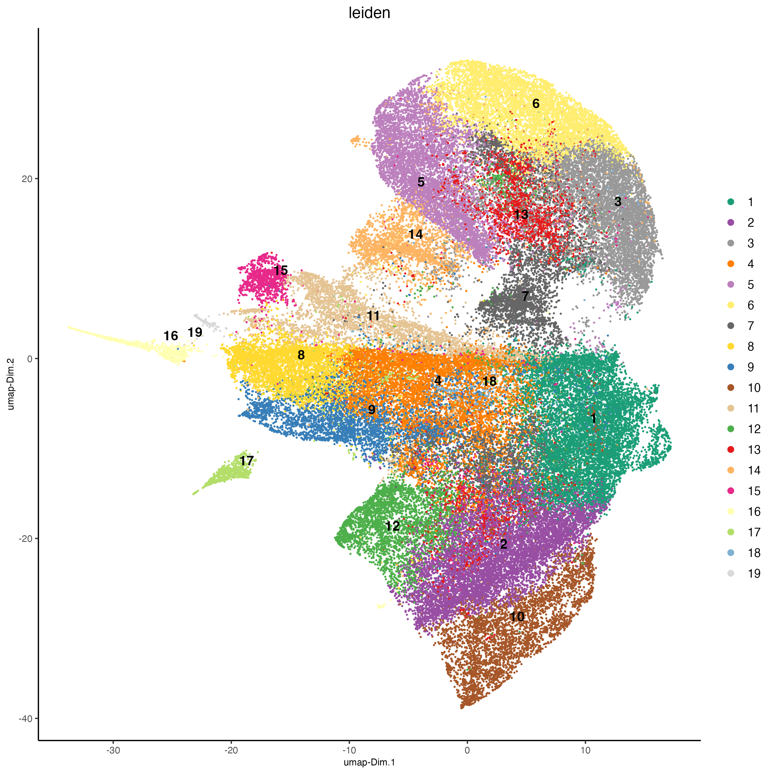
spatPlot(gobject = codex_tesTRUE,
         cell_color = "leiden",
         point_shape = "no_border",
         point_size = 0.2,
         cell_color_code = leiden_colors,
         coord_fix_ratio = 1,
         label_size = 2,
         legend_text = 5,
         legend_symbol_size = 2,
         save_param = list(save_name = "4_b_spatplot"))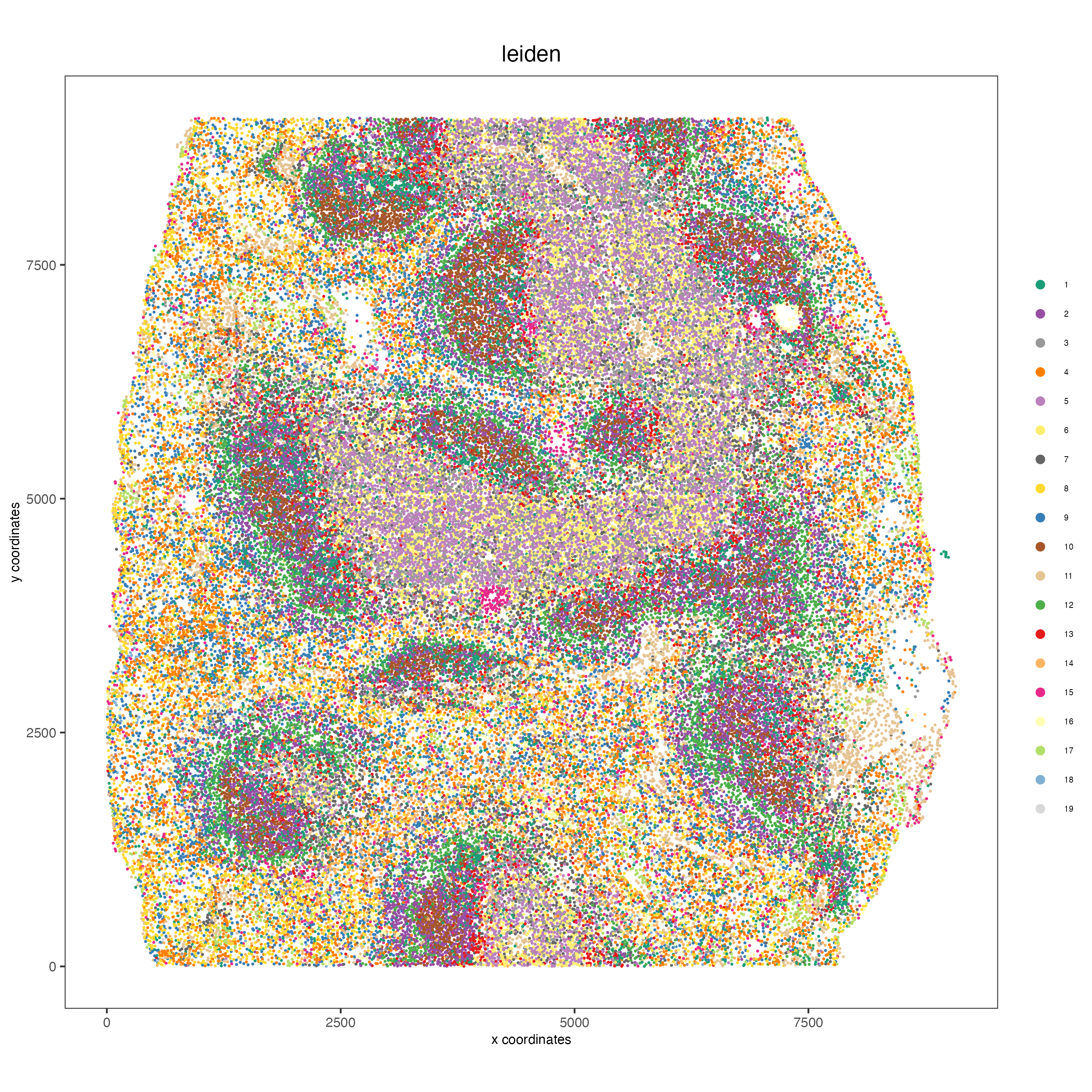
7 Co-visualize
spatDimPlot2D(gobject = codex_tesTRUE,
              cell_color = "leiden",
              spat_point_shape = "no_border",
              spat_point_size = 0.2,
              dim_point_shape = "no_border",
              dim_point_size = 0.2,
              cell_color_code = leiden_colors,
              plot_alignment = "horizontal",
              save_param = list(save_name = "5_a_spatdimplot"))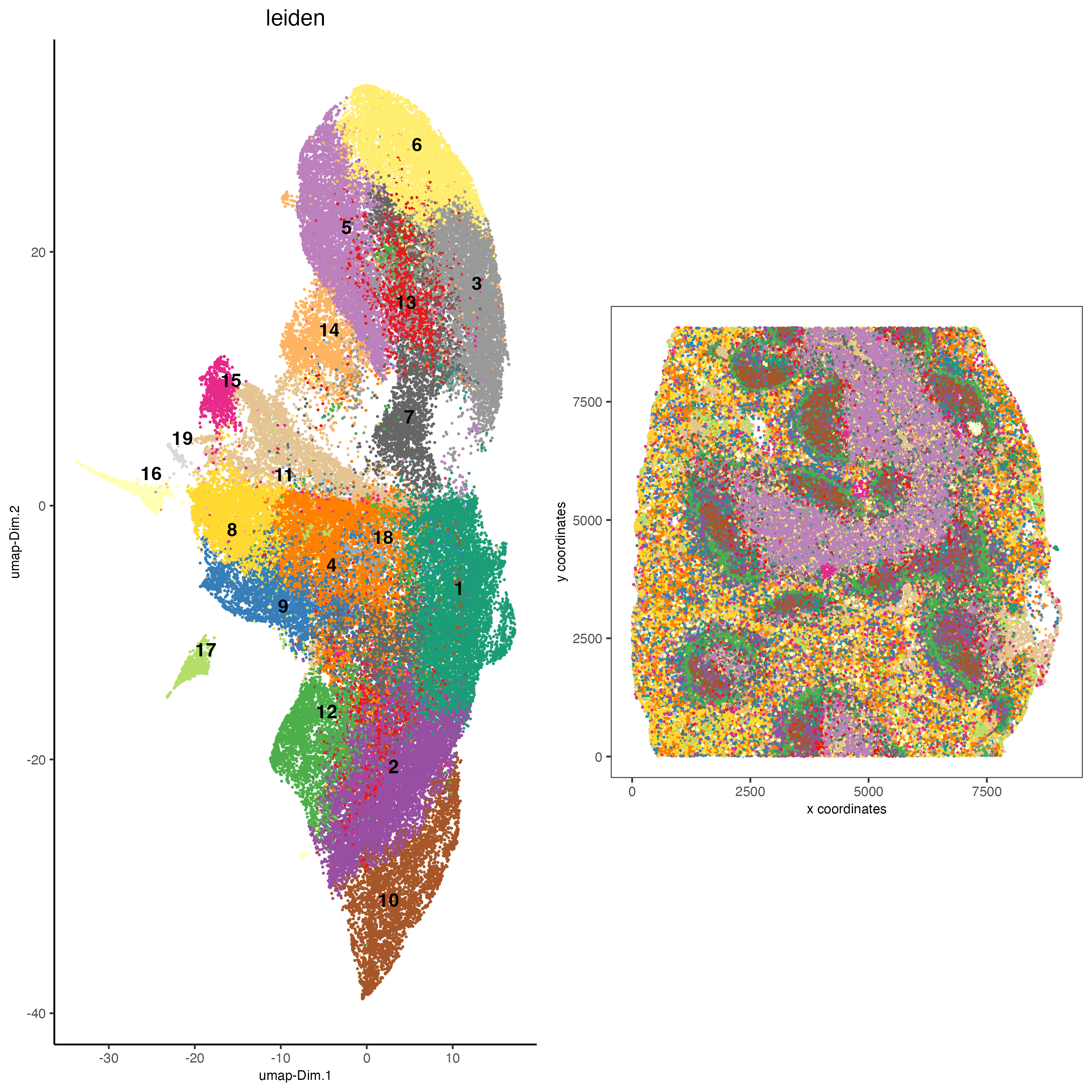
8 Differential expression
cluster_column <- "leiden"

markers_scran <- findMarkers_one_vs_all(gobject = codex_tesTRUE,
                                        method = "scran",
                                        expression_values = "normalized",
                                        cluster_column = cluster_column,
                                        min_feats = 3)

topgenes_scran <- unique(markers_scran[, head(.SD, 5), by = "cluster"][["feats"]])

plotMetaDataHeatmap(codex_tesTRUE,
                    expression_values = "normalized",
                    metadata_cols = cluster_column,
                    selected_feats = topgenes_scran,
                    y_text_size = 8,
                    show_values = "zscores_rescaled",
                    save_param = list(save_name = "6_a_metaheatmap"))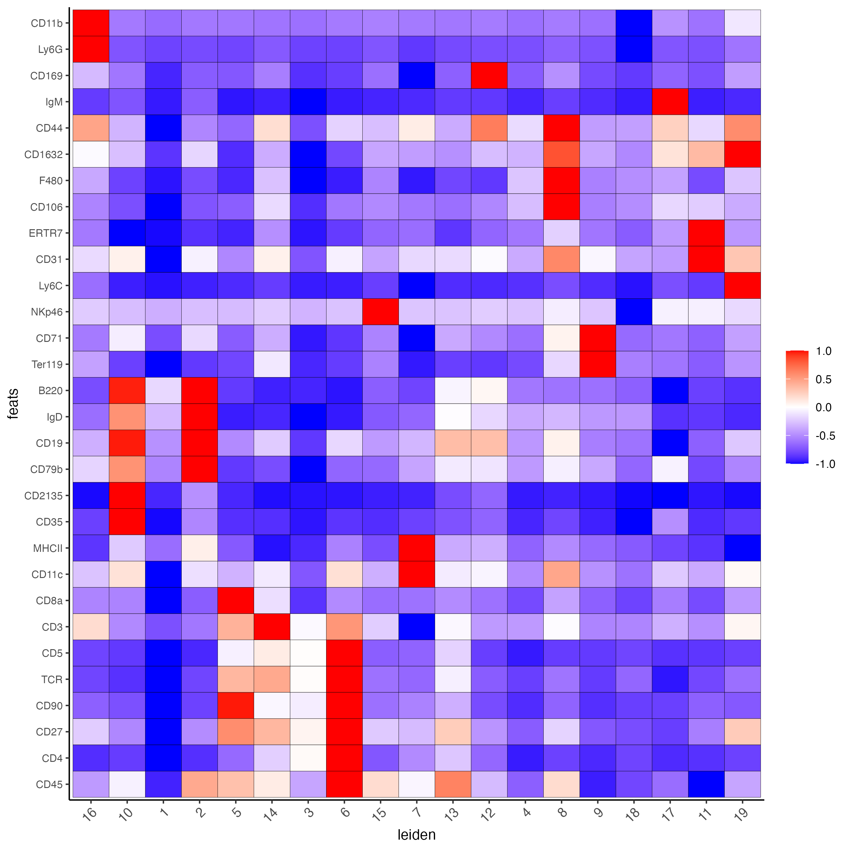
topgenes_scran <- markers_scran[, head(.SD, 1), by = "cluster"]$feats

violinPlot(codex_tesTRUE,
           feats = unique(topgenes_scran)[1:8],
           cluster_column = cluster_column,
           strip_text = 8,
           strip_position = "right",
           save_param = list(save_name = "6_b_violinplot"))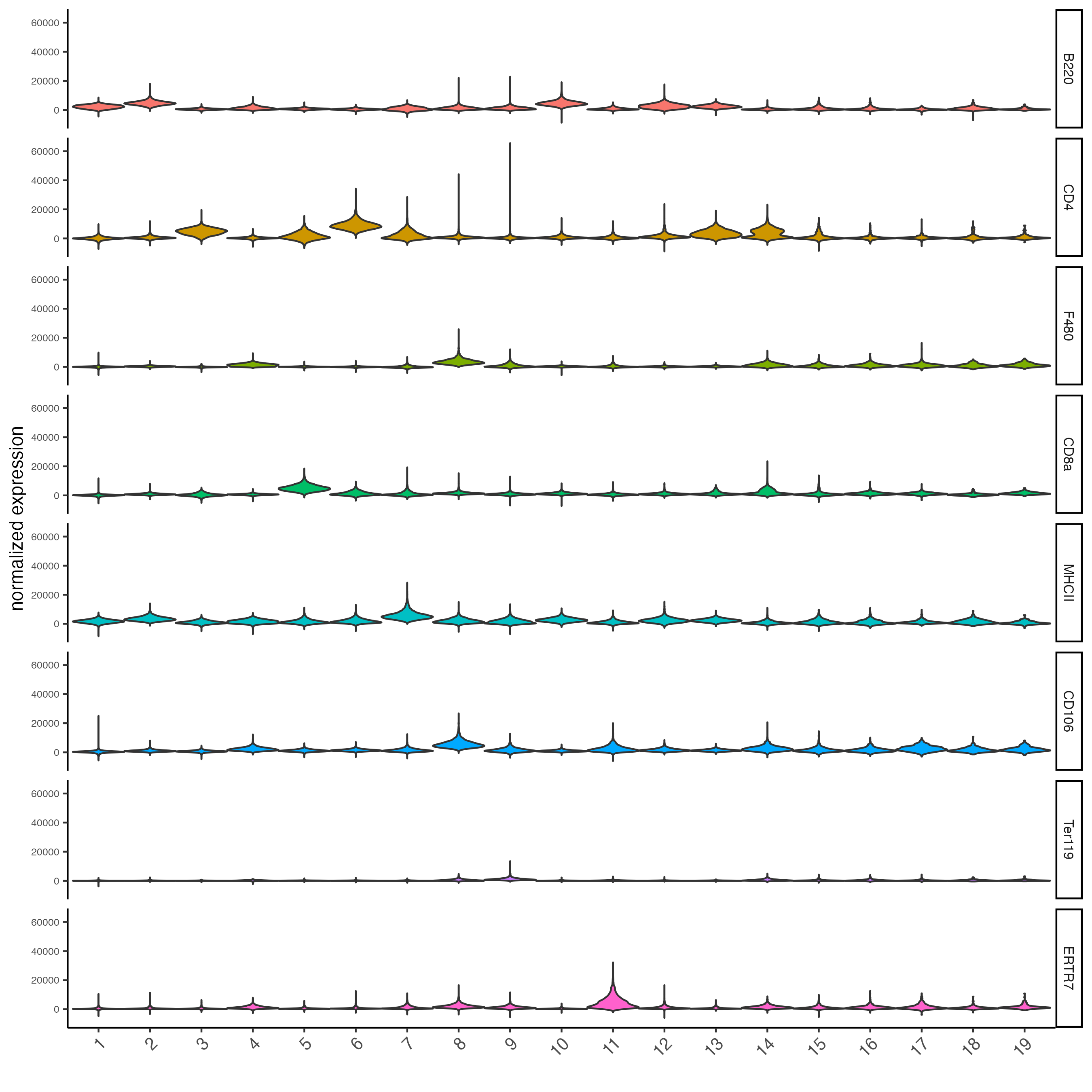
# gini
markers_gini <- findMarkers_one_vs_all(gobject = codex_tesTRUE,
                                       method = "gini",
                                       expression_values = "normalized",
                                       cluster_column = cluster_column,
                                       min_feats = 5)

topgenes_gini <- unique(markers_gini[, head(.SD, 5), by = "cluster"][["feats"]])

plotMetaDataHeatmap(codex_tesTRUE,
                    expression_values = "normalized",
                    metadata_cols = cluster_column,
                    selected_feats = topgenes_gini,
                    show_values = "zscores_rescaled",
                    save_param = list(save_name = "6_c_metaheatmap"))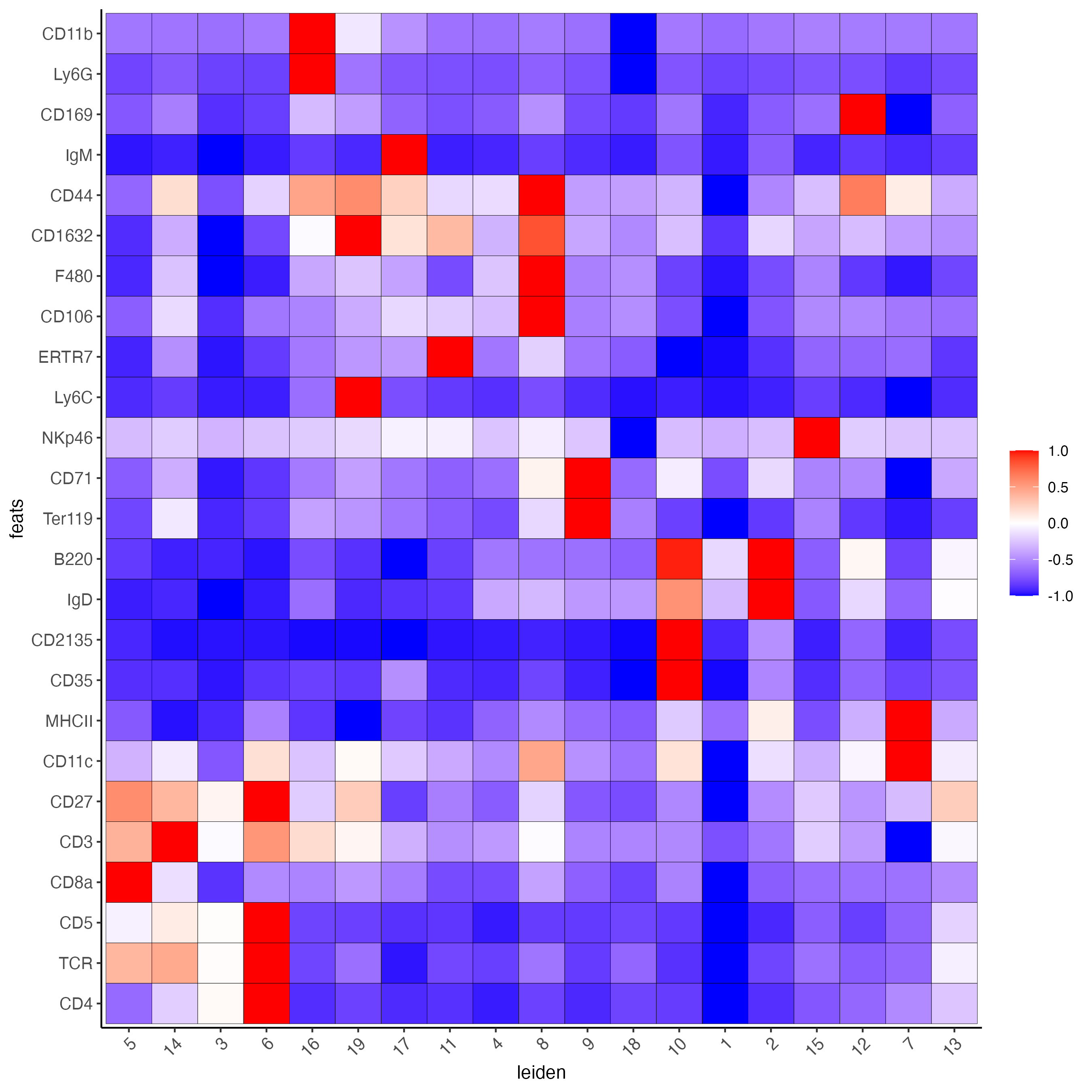
topgenes_gini <- markers_gini[, head(.SD, 1), by = "cluster"]$feats

violinPlot(codex_tesTRUE,
           feats = unique(topgenes_gini),
           cluster_column = cluster_column,
           strip_text = 8,
           strip_position = "right",
           save_param = list(save_name = "6_d_violinplot"))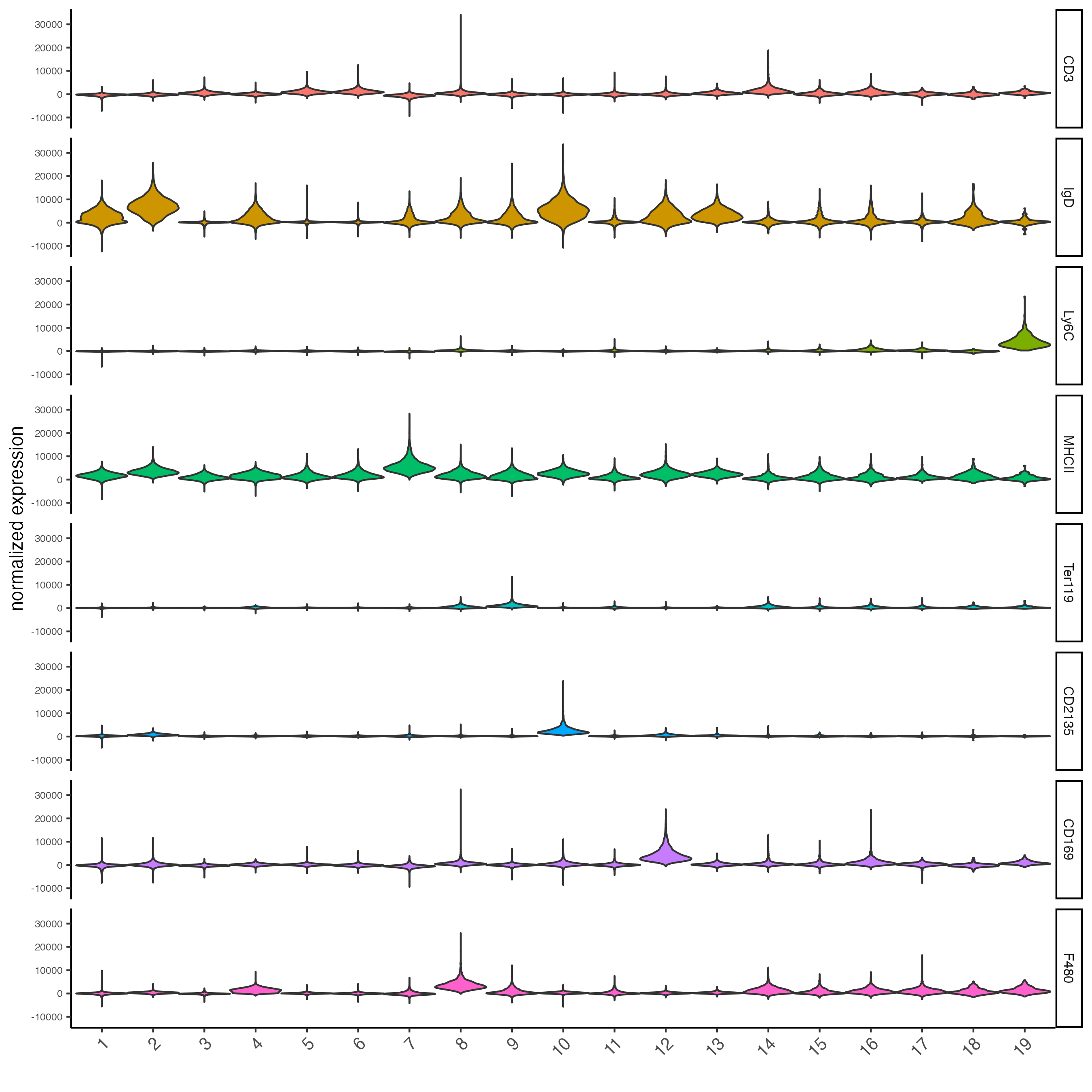
9 Cell type annotation
clusters_cell_types <- c("naive B cells", "B cells", "B cells", "naive B cells",
                         "B cells", "macrophages", "erythroblasts",
                         "erythroblasts", "erythroblasts", "CD8 + T cells",
                         "Naive T cells", "CD4+ T cells", "Naive T cells",
                         "CD4+ T cells", "Dendritic cells", "NK cells",
                         "Dendritic cells", "Plasma cells", "endothelial cells",
                         "monocytes")

names(clusters_cell_types) <- c(2, 15, 13, 5, 8, 9, 19, 1, 10, 3, 12, 14, 4, 6,
                                7, 16, 17, 18, 11, 20)

codex_test <- annotateGiotto(gobject = codex_tesTRUE,
                             annotation_vector = clusters_cell_types,
                             cluster_column = "leiden",
                             name = "cell_types")

plotUMAP(gobject = codex_tesTRUE,
         cell_color = "cell_types",
         point_shape = "no_border",
         point_size = 0.2,
         show_center_label = FALSE,
         label_size = 2,
         legend_text = 5,
         legend_symbol_size = 2,
         save_param = list(save_name = "7_a_umap_celltypes"))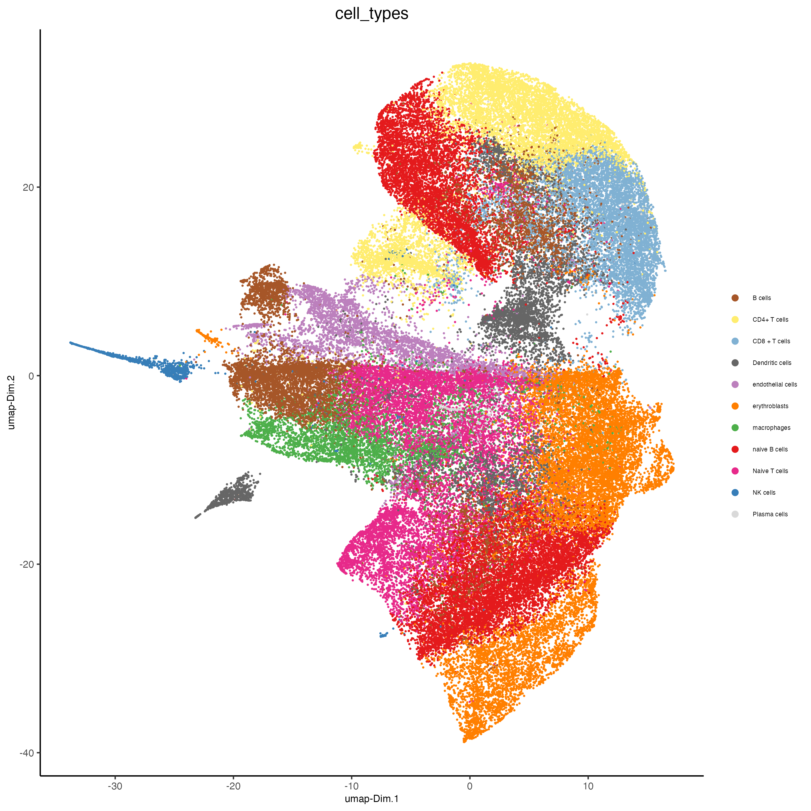
Or, this dataset comes with the imaging phenotype annotation
plotUMAP(gobject = codex_tesTRUE,
         cell_color = "Imaging_phenotype_cell_type",
         point_shape = "no_border",
         point_size = 0.2,
         show_center_label = FALSE,
         label_size = 2,
         legend_text = 5,
         legend_symbol_size = 2,
         save_param = list(save_name = "7_b_umap"))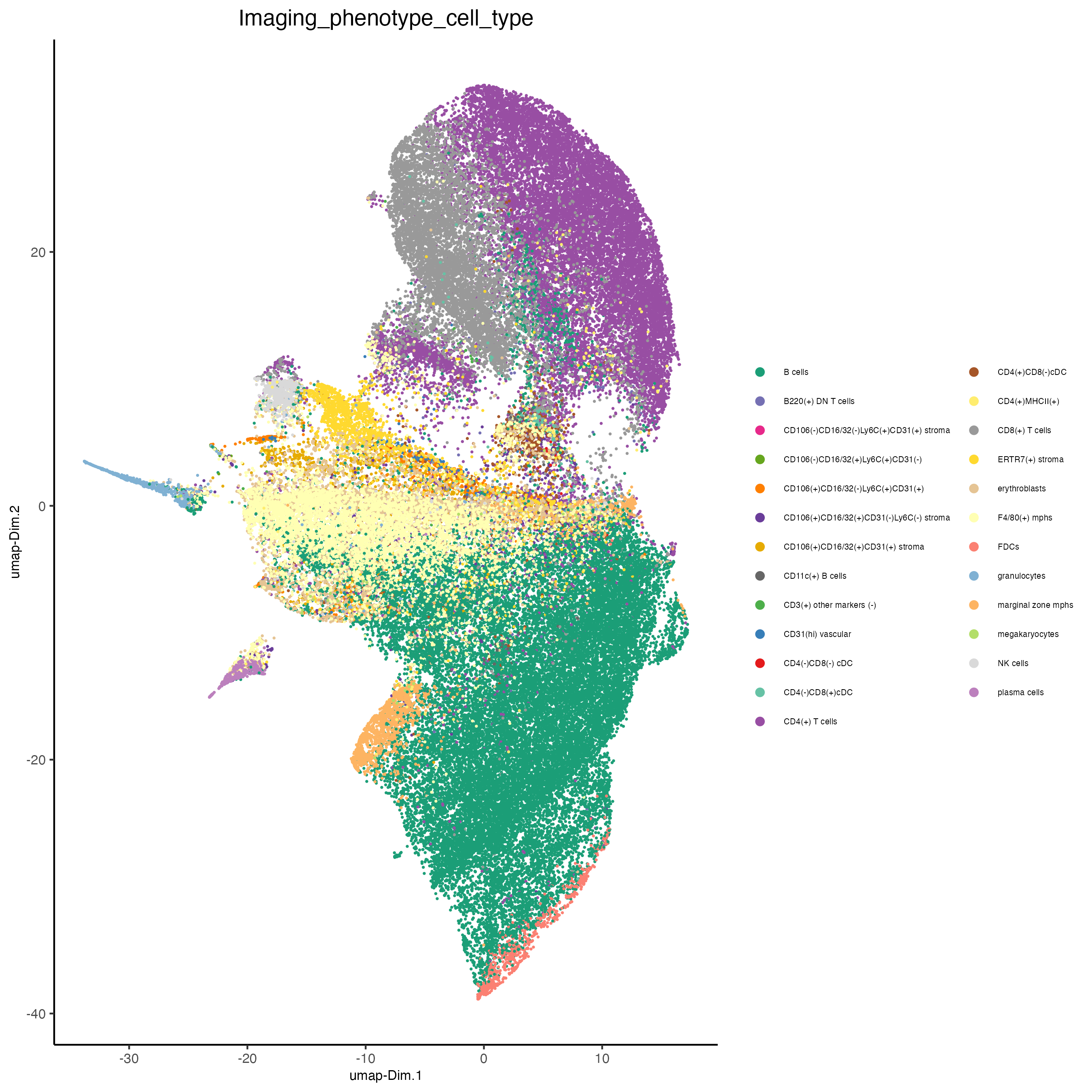
spatPlot(gobject = codex_tesTRUE,
         cell_color = "Imaging_phenotype_cell_type",
         point_shape = "no_border",
         point_size = 0.2,
         coord_fix_ratio = 1,
         label_size = 2,
         legend_text = 5,
         legend_symbol_size = 2,
         save_param = list(save_name = "7_c_spatplot"))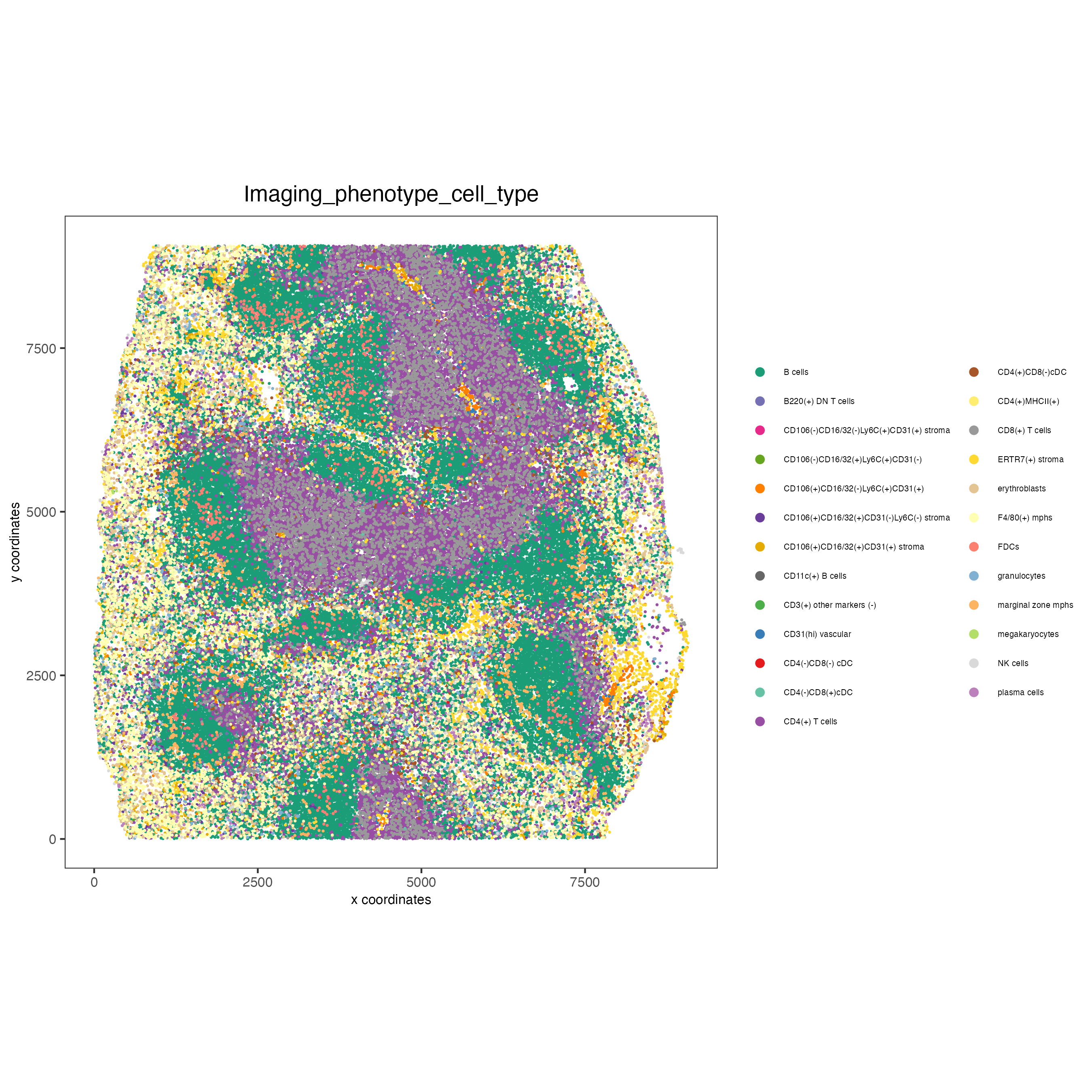
10 Visualize cell types and gene expression in selected zones
cell_metadatadata <- pDataDT(codex_test)
subset_cell_ids <- cell_metadatadata[sample_Xtile_Ytile=="BALBc-3_X04_Y08"]$cell_ID

codex_test_zone1 <- subsetGiotto(codex_tesTRUE,
                                 cell_ids = subset_cell_ids)

plotUMAP(gobject = codex_test_zone1,
         cell_color = "Imaging_phenotype_cell_type",
         point_shape = "no_border",
         point_size = 1,
         show_center_label = FALSE,
         label_size = 2,
         legend_text = 5,
         legend_symbol_size = 2,
         save_param = list(save_name = "8_a_umap"))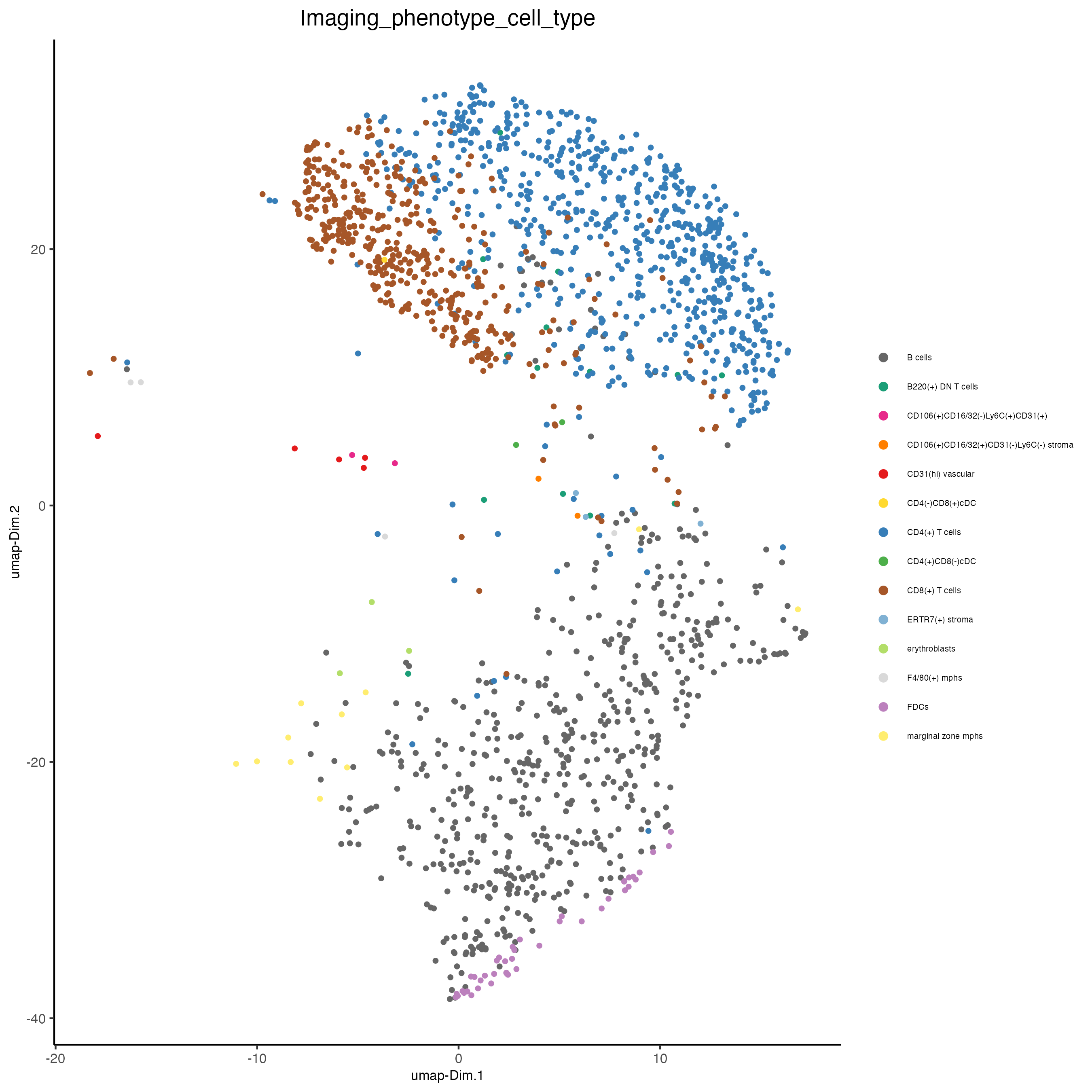
spatPlot(gobject = codex_test_zone1,
         cell_color = "Imaging_phenotype_cell_type",
         point_shape = "no_border",
         point_size = 1,
         coord_fix_ratio = 1,
         label_size = 2,
         legend_text = 5,
         legend_symbol_size = 2,
         save_param = list(save_name = "8_b_spatplot"))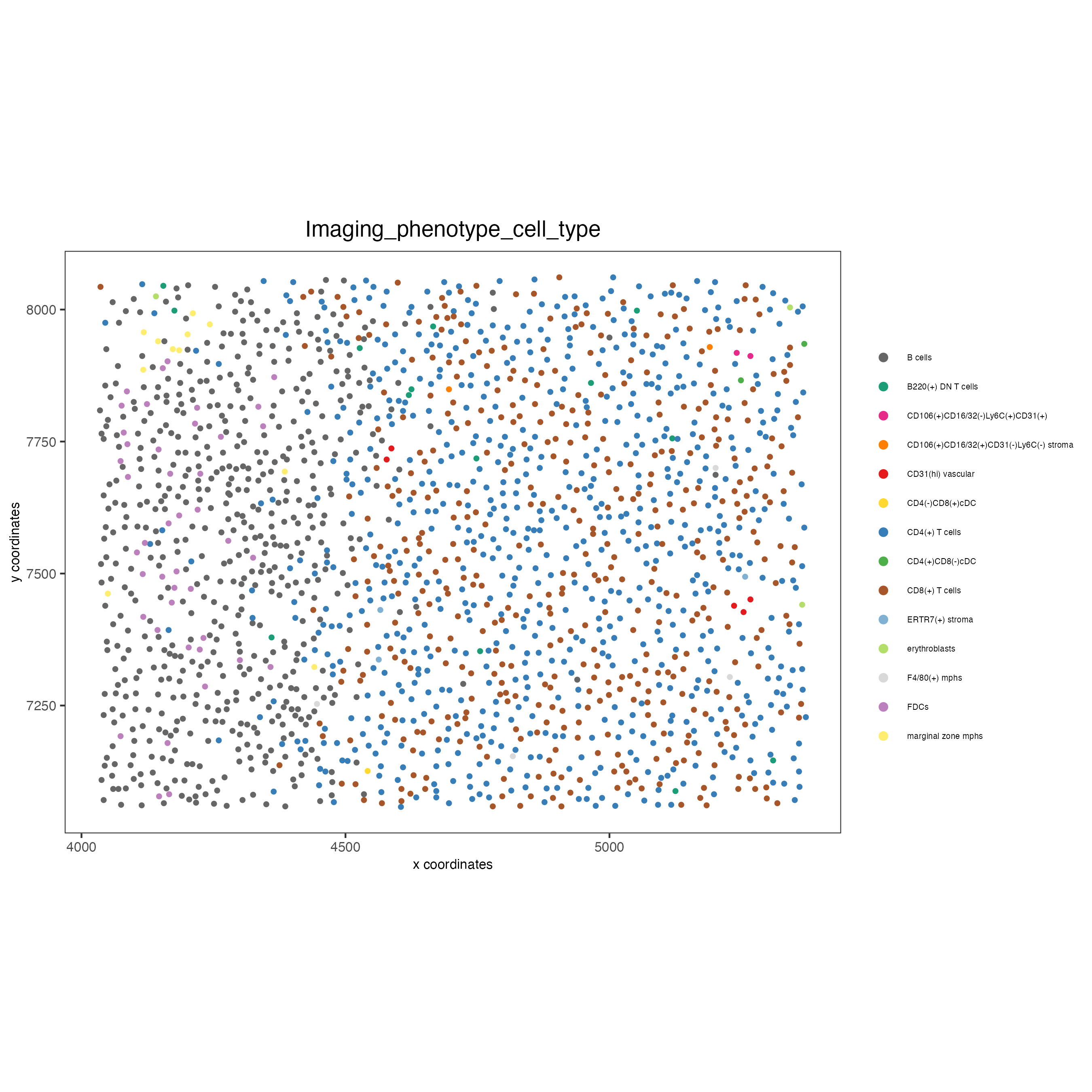
spatDimFeatPlot2D(codex_test_zone1,
                  expression_values = "scaled",
                  feats = c("CD8a","CD19"),
                  spat_point_shape = "no_border",
                  dim_point_shape = "no_border",
                  cell_color_gradient = c("darkblue", "white", "red"),
                  save_param = list(save_name = "8_c_spatdimplot"))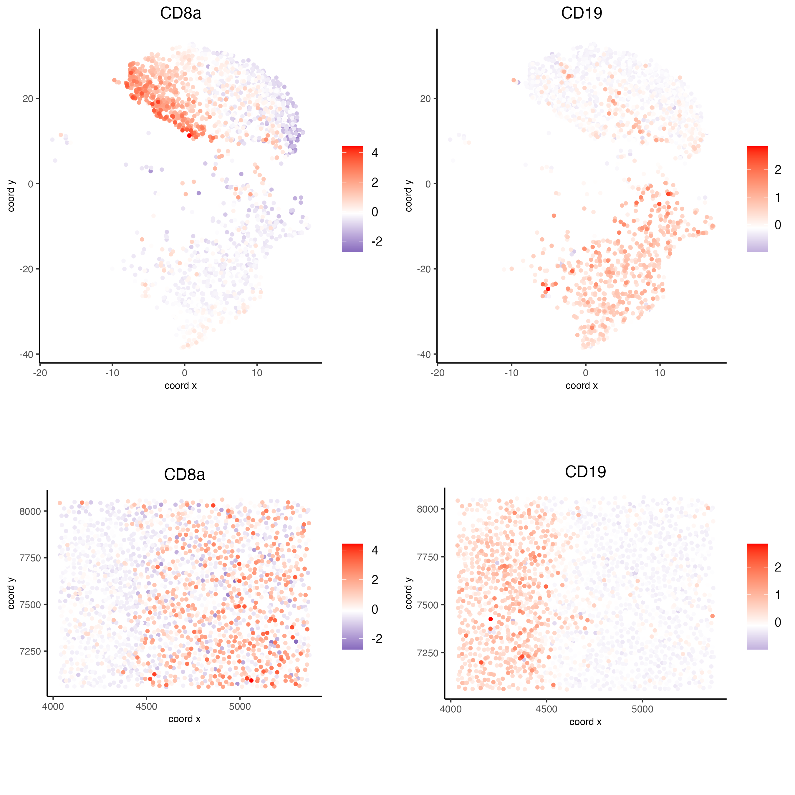
Test on another region:
cell_metadatadata <- pDataDT(codex_test)

subset_cell_ids <- cell_metadatadata[sample_Xtile_Ytile=="BALBc-3_X04_Y03"]$cell_ID

codex_test_zone2 <- subsetGiotto(codex_tesTRUE,
                                 cell_ids = subset_cell_ids)

plotUMAP(gobject = codex_test_zone2,
         cell_color = "Imaging_phenotype_cell_type",
         point_shape = "no_border",
         point_size = 1,
         show_center_label = FALSE,
         label_size = 2,
         legend_text = 5,
         legend_symbol_size = 2,
         save_param = list(save_name = "8_d_umap"))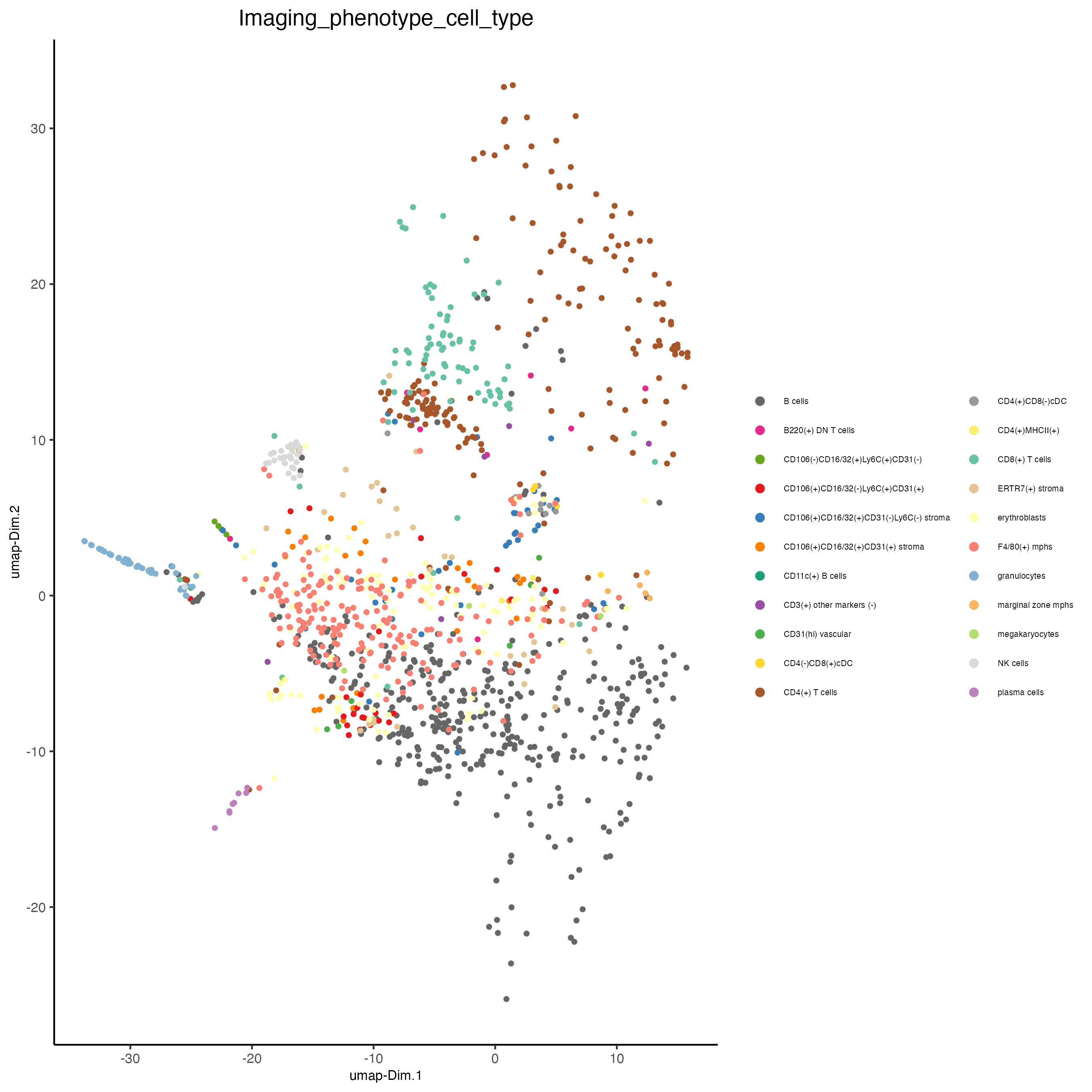
spatPlot(gobject = codex_test_zone2,
         cell_color = "Imaging_phenotype_cell_type",
         point_shape = "no_border",
         point_size = 1,
         coord_fix_ratio = 1,
         label_size = 2,
         legend_text = 5,
         legend_symbol_size = 2,
         save_param = list(save_name = "8_e_spatPlot"))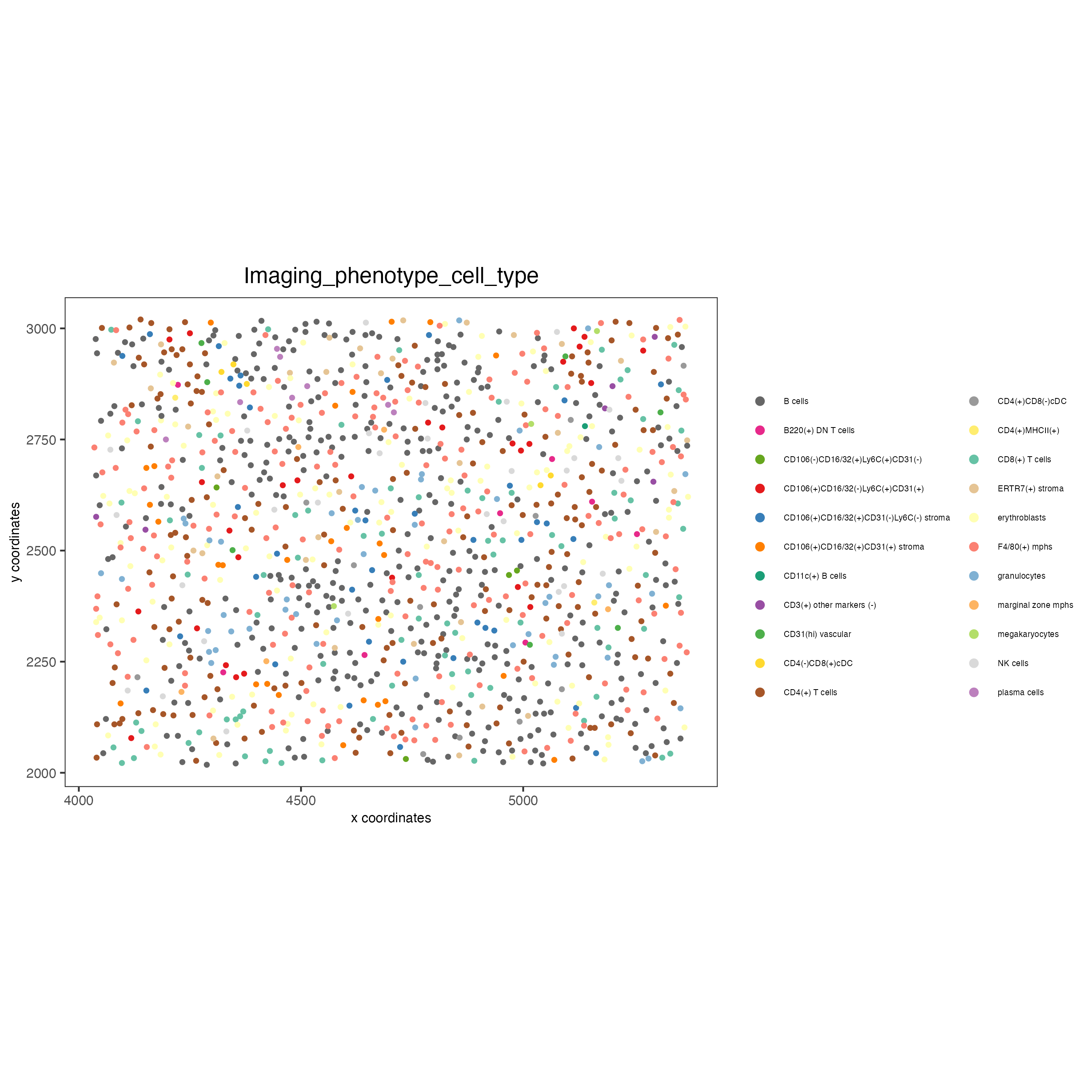
spatDimFeatPlot2D(codex_test_zone2,
                  expression_values = "scaled",
                  feats = c("CD4", "CD106"),
                  spat_point_shape = "no_border",
                  dim_point_shape = "no_border",
                  cell_color_gradient = c("darkblue", "white", "red"),
                  save_param = list(save_name = "8_f_spatdimgeneplot"))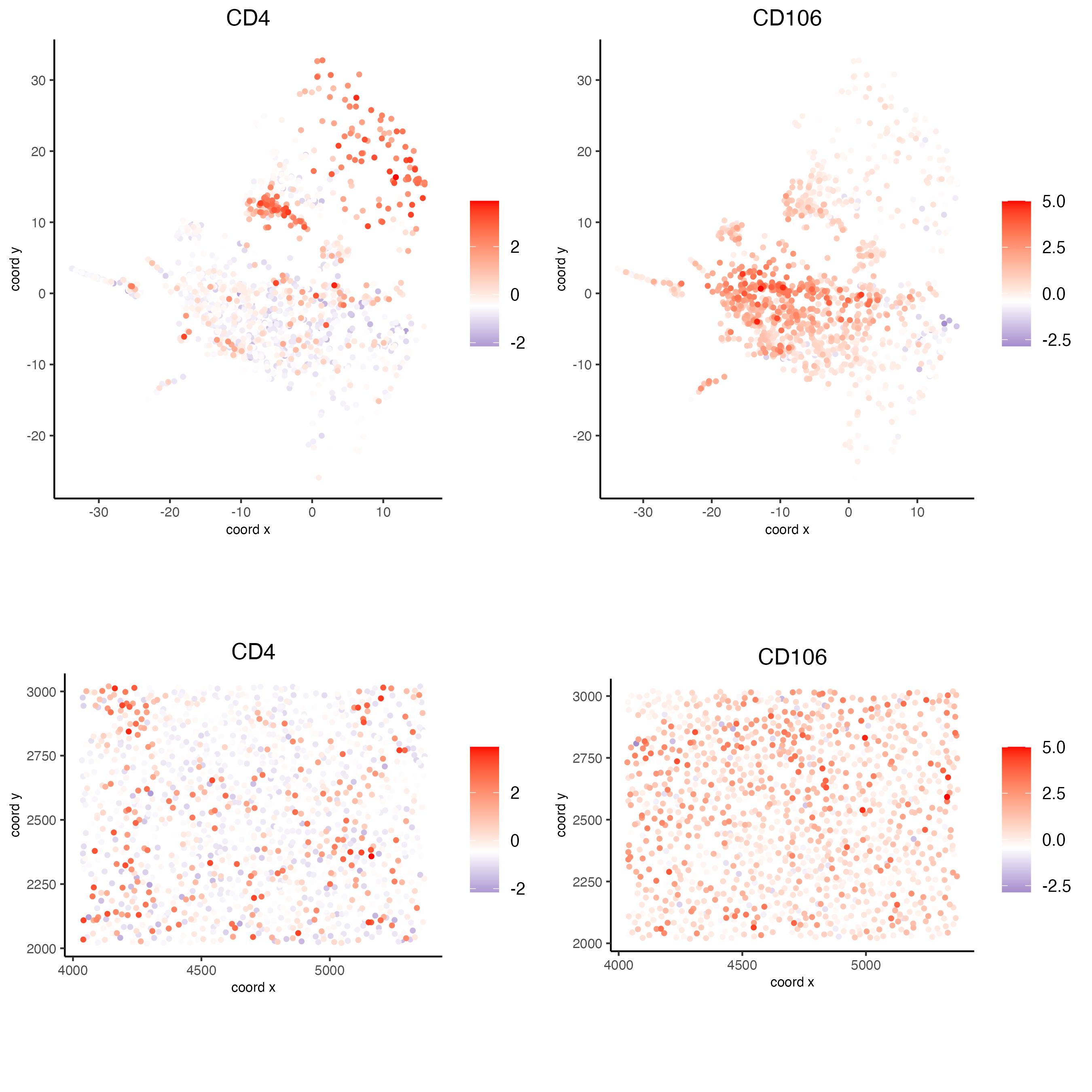
11 Session info
R version 4.3.2 (2023-10-31)
Platform: x86_64-apple-darwin20 (64-bit)
Running under: macOS Sonoma 14.3.1

Matrix products: default
BLAS:   /System/Library/Frameworks/Accelerate.framework/Versions/A/Frameworks/vecLib.framework/Versions/A/libBLAS.dylib
LAPACK: /Library/Frameworks/R.framework/Versions/4.3-x86_64/Resources/lib/libRlapack.dylib;  LAPACK version 3.11.0

locale:
[1] en_US.UTF-8/en_US.UTF-8/en_US.UTF-8/C/en_US.UTF-8/en_US.UTF-8

time zone: America/New_York
tzcode source: internal

attached base packages:
[1] stats     graphics  grDevices utils     datasets  methods   base

other attached packages:
[1] GiottoData_0.2.6.2 GiottoUtils_0.1.5  Giotto_4.0.2       GiottoClass_0.1.3

loaded via a namespace (and not attached):
  [1] colorRamp2_0.1.0            bitops_1.0-7                rlang_1.1.3
  [4] magrittr_2.0.3              RcppAnnoy_0.0.22            matrixStats_1.2.0
  [7] compiler_4.3.2              DelayedMatrixStats_1.24.0   png_0.1-8
 [10] systemfonts_1.0.5           vctrs_0.6.5                 pkgconfig_2.0.3
 [13] SpatialExperiment_1.12.0    crayon_1.5.2                fastmap_1.1.1
 [16] backports_1.4.1             magick_2.8.2                XVector_0.42.0
 [19] scuttle_1.12.0              labeling_0.4.3              utf8_1.2.4
 [22] rmarkdown_2.25              ragg_1.2.7                  bluster_1.12.0
 [25] xfun_0.42                   beachmat_2.18.0             zlibbioc_1.48.0
 [28] GenomeInfoDb_1.38.6         jsonlite_1.8.8              flashClust_1.01-2
 [31] pak_0.7.1                   DelayedArray_0.28.0         BiocParallel_1.36.0
 [34] terra_1.7-71                irlba_2.3.5.1               parallel_4.3.2
 [37] cluster_2.1.6               R6_2.5.1                    RColorBrewer_1.1-3
 [40] limma_3.58.1                reticulate_1.35.0           GenomicRanges_1.54.1
 [43] estimability_1.4.1          Rcpp_1.0.12                 SummarizedExperiment_1.32.0
 [46] knitr_1.45                  R.utils_2.12.3              IRanges_2.36.0
 [49] igraph_2.0.1.1              Matrix_1.6-5                tidyselect_1.2.0
 [52] rstudioapi_0.15.0           abind_1.4-5                 yaml_2.3.8
 [55] codetools_0.2-19            lattice_0.22-5              tibble_3.2.1
 [58] Biobase_2.62.0              withr_3.0.0                 evaluate_0.23
 [61] pillar_1.9.0                MatrixGenerics_1.14.0       checkmate_2.3.1
 [64] DT_0.31                     stats4_4.3.2                dbscan_1.1-12
 [67] generics_0.1.3              RCurl_1.98-1.14             S4Vectors_0.40.2
 [70] ggplot2_3.4.4               sparseMatrixStats_1.14.0    munsell_0.5.0
 [73] scales_1.3.0                gtools_3.9.5                xtable_1.8-4
 [76] leaps_3.1                   glue_1.7.0                  metapod_1.10.1
 [79] emmeans_1.10.0              scatterplot3d_0.3-44        tools_4.3.2
 [82] GiottoVisuals_0.1.4         BiocNeighbors_1.20.2        data.table_1.15.0
 [85] ScaledMatrix_1.10.0         locfit_1.5-9.8              scran_1.30.2
 [88] mvtnorm_1.2-4               cowplot_1.1.3               grid_4.3.2
 [91] edgeR_4.0.14                colorspace_2.1-0            SingleCellExperiment_1.24.0
 [94] GenomeInfoDbData_1.2.11     BiocSingular_1.18.0         rsvd_1.0.5
 [97] cli_3.6.2                   textshaping_0.3.7           fansi_1.0.6
[100] S4Arrays_1.2.0              dplyr_1.1.4                 uwot_0.1.16
[103] gtable_0.3.4                R.methodsS3_1.8.2           digest_0.6.34
[106] progressr_0.14.0            BiocGenerics_0.48.1         dqrng_0.3.2
[109] SparseArray_1.2.3           ggrepel_0.9.5               FactoMineR_2.9
[112] rjson_0.2.21                htmlwidgets_1.6.4           farver_2.1.1
[115] htmltools_0.5.7             R.oo_1.26.0                 lifecycle_1.0.4
[118] multcompView_0.1-9          statmod_1.5.0               MASS_7.3-60.0.1