1 Explanation
This tutorial walks through saving spatial data in plots. Please see the Configuration and Giotto Object vignettes before walking through this tutorial.
R/Posit and Giotto provide different ways to save spatial data. Here, a giottoObject will be created without using giottoInstructions so that the save parameters for plotting functions within Giotto as well as the default saving methods built into R/Posit may be emphasized here. Note that for plotting functions, all parameters available to the save_param argument may be found by running showSaveParameters().
2 Start Giotto
# Ensure Giotto Suite is installed
if(!"Giotto" %in% installed.packages()) {
  pak::pkg_install("drieslab/Giotto")
}

library(Giotto)

# Ensure Giotto Data is installed
if(!"GiottoData" %in% installed.packages()) {
  pak::pkg_install("drieslab/GiottoData")
}

library(GiottoData)

# Ensure the Python environment for Giotto has been installed
genv_exists <- checkGiottoEnvironment()
if(!genv_exists){
  # The following command need only be run once to install the Giotto environment
  installGiottoEnvironment()
}
3 Create a Giotto object
Since the focus of this vignette is saving methods, the giottoObject will not be created with giottoInstructions. See Giotto Object for further intuition on working with a giottoObject that has been provided instructions.
data_path <- "/path/to/data/"

# Download dataset
getSpatialDataset(dataset = "osmfish_SS_cortex",
                  directory = data_path,
                  method = "wget")

# Specify path to files
osm_exprs <- paste0(data_path, "osmFISH_prep_expression.txt")
osm_locs <- paste0(data_path, "osmFISH_prep_cell_coordinates.txt")
meta_path <- paste0(data_path, "osmFISH_prep_cell_metadata.txt")

## CREATE GIOTTO OBJECT with expression data and location data
my_gobject <- createGiottoObject(expression = osm_exprs,
                                spatial_locs = osm_locs)

metadata <- data.table::fread(file = meta_path)
my_gobject <- addCellMetadata(my_gobject,
                             new_metadata = metadata,
                             by_column = TRUE,
                             column_cell_ID = "CellID")
4 Standard R Save Methods
Note that by default, plotting functions will return a plot object that may be saved or further manipulated. Manually save plot as a PDF in the current working directory:
save_path <- paste0(getwd(), "/first_plot.pdf")
library(ggplot2)

# This function serves only to ensure the following lines run consecutively.
save_pdf_plot = function(){
  pdf(file = save_path, width = 7, height = 7)
  pl = spatPlot(my_gobject)
  dev.off()
}

save_pdf_plot()

### Plot clusters, edit plot object, then save using the ggplot add-on, cowplot:
mypl <- spatPlot(gobject = my_gobject,
                 cell_color = "ClusterName")
# Add a black background
mypl <- mypl + theme(panel.background = element_rect(fill ="black"),
                     panel.grid = element_blank())

# Add a legend
mypl <- mypl + guides(fill = guide_legend(override.aes = list(size=5)))

# Save in the current working directory
cowplot::save_plot(plot = mypl,
                   filename = "clusters_black.png",
                   path = getwd(),
                   device = png(),
                   dpi = 300,
                   base_height = 10,
                   base_width = 10)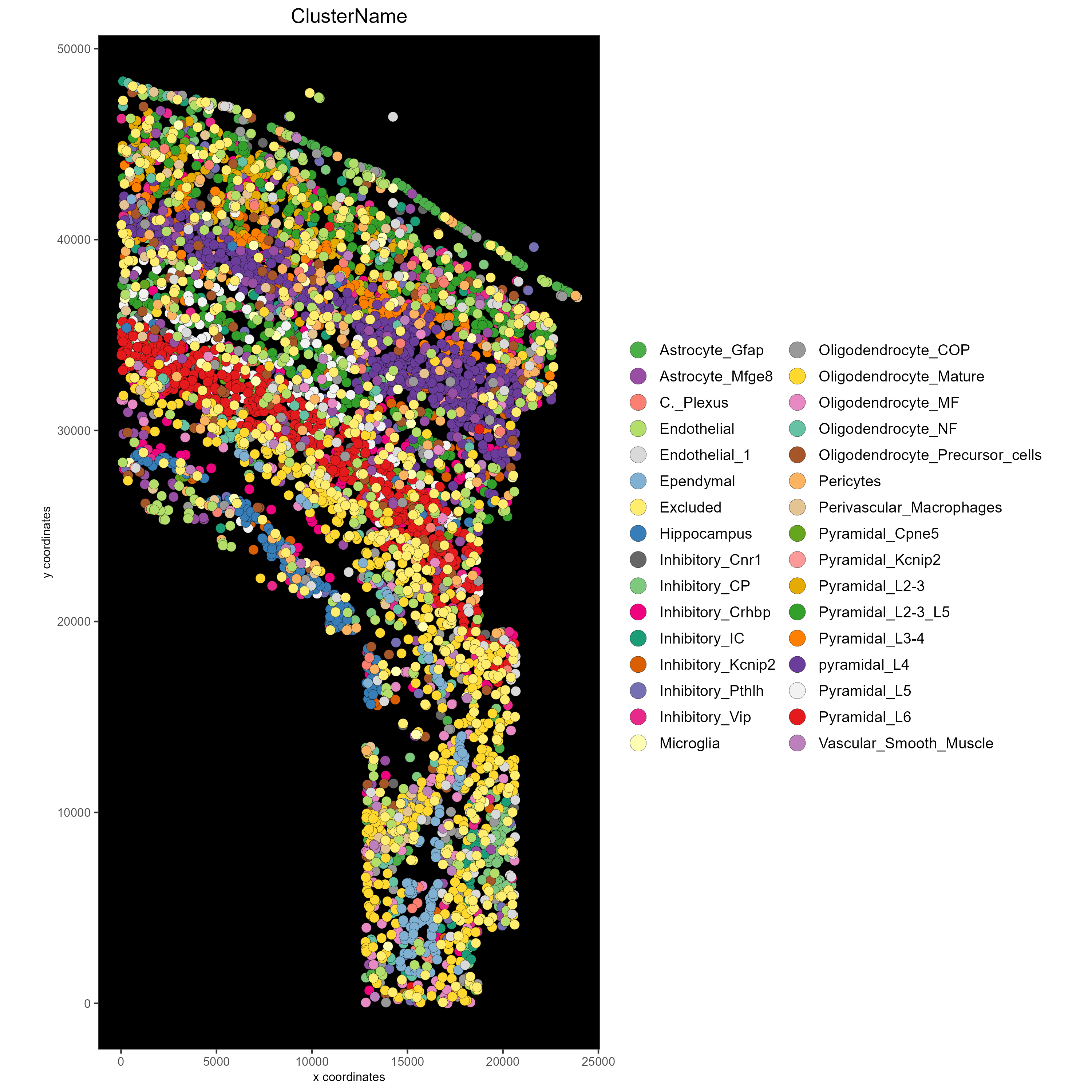
5 Save Plot Directly to the Default Folder
The default save folder is the current working directory. This will be the case if instructions are not provided, or if a save_dir is not specified within giottoInstructions. See the createGiottoInstructions documentation and Giotto Object for default arguments and more details.
spatPlot(my_gobject,
         cell_color = "ClusterName",
         save_plot = TRUE)
6 Save plot Directly, but Overwrite Default Save Parameters
In this example, assume it is desired that the plot is: - Shown in the console - Not returned as an object from the plotting function call -Saved in a subdirectory of the current working directory as a .png file with a dpi of 200, height of 9 inches, and width of 9 inches. - Saved with the file name “my_name”
See Giotto Object for more details.
Run the command showSaveParameters() to see all available parameters.
# Specify new subdirectory name
results_folder <- "/path/to/results/"

# Plot clusters, create, and save to a new subdirectory with specifications above.
spatPlot(my_gobject,
         cell_color = "ClusterName",
         save_plot = TRUE,
         return_plot = FALSE,
         save_param = list(save_folder = results_folder, # Create subdirectory
                           save_name = "my_name",
                           save_format = "png",
                           units = "in",
                           base_height = 9,
                           base_width = 9))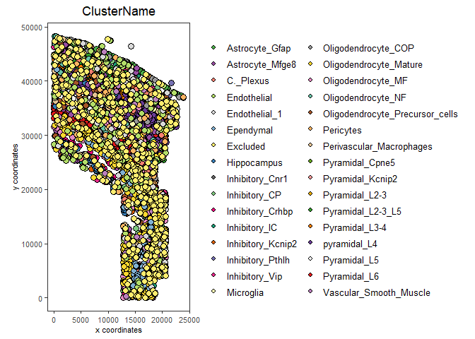
7 Just View the Plot
See Giotto Object for more details.
Set both save_plot and return_plot to FALSE.
# Plot without saving
spatPlot(my_gobject,
         cell_color = "ClusterName",
         save_plot = FALSE,
         return_plot = FALSE,
         show_plot = TRUE)
8 Just save the plot (FASTEST for large datasets!)
See Giotto Object for more details.
Set show_plot and return_plot to FALSE, set save_plot to TRUE.
9 Session Info
R version 4.2.2 (2022-10-31 ucrt)
Platform: x86_64-w64-mingw32/x64 (64-bit)
Running under: Windows 10 x64 (build 22621)

Matrix products: default

locale:
[1] LC_COLLATE=English_United States.utf8
[2] LC_CTYPE=English_United States.utf8
[3] LC_MONETARY=English_United States.utf8
[4] LC_NUMERIC=C
[5] LC_TIME=English_United States.utf8

attached base packages:
[1] stats     graphics  grDevices utils     datasets  methods   base

other attached packages:
[1] ggplot2_3.4.1    GiottoData_0.2.1 Giotto_3.2.1

loaded via a namespace (and not attached):
[1] Rcpp_1.0.10        RColorBrewer_1.1-3 pillar_1.9.0       compiler_4.2.2
[5] tools_4.2.2        digest_0.6.30      jsonlite_1.8.3     evaluate_0.20
[9] lifecycle_1.0.3    tibble_3.2.1       gtable_0.3.3       lattice_0.20-45
[13] png_0.1-7          pkgconfig_2.0.3    rlang_1.1.0        Matrix_1.5-1
[17] cli_3.4.1          rstudioapi_0.14    parallel_4.2.2     yaml_2.3.7
[21] xfun_0.38          fastmap_1.1.0      terra_1.7-18       withr_2.5.0
[25] dplyr_1.1.1        knitr_1.42         systemfonts_1.0.4  rappdirs_0.3.3
[29] generics_0.1.3     vctrs_0.6.1        cowplot_1.1.1      grid_4.2.2
[33] tidyselect_1.2.0   reticulate_1.26    glue_1.6.2         data.table_1.14.6
[37] R6_2.5.1           textshaping_0.3.6  fansi_1.0.4        rmarkdown_2.21
[41] farver_2.1.1       magrittr_2.0.3     scales_1.2.1       codetools_0.2-18
[45] htmltools_0.5.4    colorspace_2.1-0   ragg_1.2.4         labeling_0.4.2
[49] utf8_1.2.3         munsell_0.5.0