Visium CytAssist Multi-omics Human Glioblastoma
Source:vignettes/visium_cytassist_human_glioblastoma.Rmd
visium_cytassist_human_glioblastoma.Rmd1 Dataset explanation
The Human glioblastoma (FFPE) dataset was obtained from 10x Genomics. The tissue was sectioned as described in Visium CytAssist Spatial Gene Expression for FFPE – Tissue Preparation Guide Demonstrated Protocol (CG000518). 5 µm tissue sections were placed on Superfrost glass slides, then IF stained following deparaffinization, then hard coverslipped. Sections were imaged, decoverslipped, followed by Demonstrated Protocol (CG000494).
More information about this dataset can be found here.
2 Download dataset
For running this tutorial, we need to download the expression matrix that contains both the RNA and Protein counts, as well as the spatial folder with the tissue image and spatial coordinates.
After downloading the compressed files, unzip them to access the folder structure.
dir.create("data")

download.file(url = "https://cf.10xgenomics.com/samples/spatial-exp/2.1.0/CytAssist_FFPE_Protein_Expression_Human_Glioblastoma/CytAssist_FFPE_Protein_Expression_Human_Glioblastoma_raw_feature_bc_matrix.tar.gz",
              destfile = "data/CytAssist_FFPE_Protein_Expression_Human_Glioblastoma_raw_feature_bc_matrix.tar.gz")

download.file(url = "https://cf.10xgenomics.com/samples/spatial-exp/2.1.0/CytAssist_FFPE_Protein_Expression_Human_Glioblastoma/CytAssist_FFPE_Protein_Expression_Human_Glioblastoma_spatial.tar.gz",
              destfile = "data/CytAssist_FFPE_Protein_Expression_Human_Glioblastoma_spatial.tar.gz")

untar("data/CytAssist_FFPE_Protein_Expression_Human_Glioblastoma_raw_feature_bc_matrix.tar.gz",
      exdir = "data")
untar("data/CytAssist_FFPE_Protein_Expression_Human_Glioblastoma_spatial.tar.gz",
      exdir = "data")
3 Start Giotto
Make sure you have the Giotto package and environment installed. If you have installation problems, visit the Installation guidelines and FAQ section.
# Ensure Giotto Suite is installed
if(!"Giotto" %in% installed.packages()) {
  pak::pkg_install("drieslab/Giotto")
}

# Ensure the Python environment for Giotto has been installed
genv_exists <- Giotto::checkGiottoEnvironment()

if(!genv_exists){
  # The following command need only be run once to install the Giotto environment
  Giotto::installGiottoEnvironment()
}
Use the Giotto instructions to set the behavior of the Giotto object, such as whether you prefer to save the generated plots or only visualize them. This instructions will become the default for future plotting functions, but you can also use the functions arguments to change the saving options.
library(Giotto)

# 1. set results directory
results_folder <- "/path/to/results/"

# 2. set giotto python path
# set python path to your preferred python version path
# set python path to NULL if you want to automatically install (only the 1st time) and use the giotto miniconda environment
python_path <- NULL

# 3. create giotto instructions
instructions <- createGiottoInstructions(save_dir = results_folder,
                                         save_plot = TRUE,
                                         show_plot = FALSE,
                                         return_plot = FALSE,
                                         python_path = python_path)
4 Create Giotto object
The minimum requirements are
- matrix with expression information (or path to)
- x,y(,z) coordinates for cells or spots (or path to)
createGiottoVisiumObject() will automatically detect both RNA and Protein modalities within the expression matrix creating a multi-omics Giotto object.
# Provide path to visium folder
data_path <- "/path/to/data/"

# Create Giotto object
visium <- createGiottoVisiumObject(visium_dir = data_path,
                                  expr_data = "raw",
                                  png_name = "tissue_lowres_image.png",
                                  gene_column_index = 2,
                                  instructions = instructions)
5 Processing
5.1 Filtering
The metadata of the CytAssist technology contains a column “in_tissue” that indicates whether a spot in on the tissue area (1) or not (0). We will use this column to remove all spots that don’t correspond to the tissue area.
# Subset on spots that were covered by tissue
metadata <- pDataDT(visium)
in_tissue_barcodes <- metadata[in_tissue == 1]$cell_ID

visium <- subsetGiotto(visium,
                       cell_ids = in_tissue_barcodes)

## Visualize aligned tissue
spatPlot2D(gobject = visium,
           point_alpha = 0.7)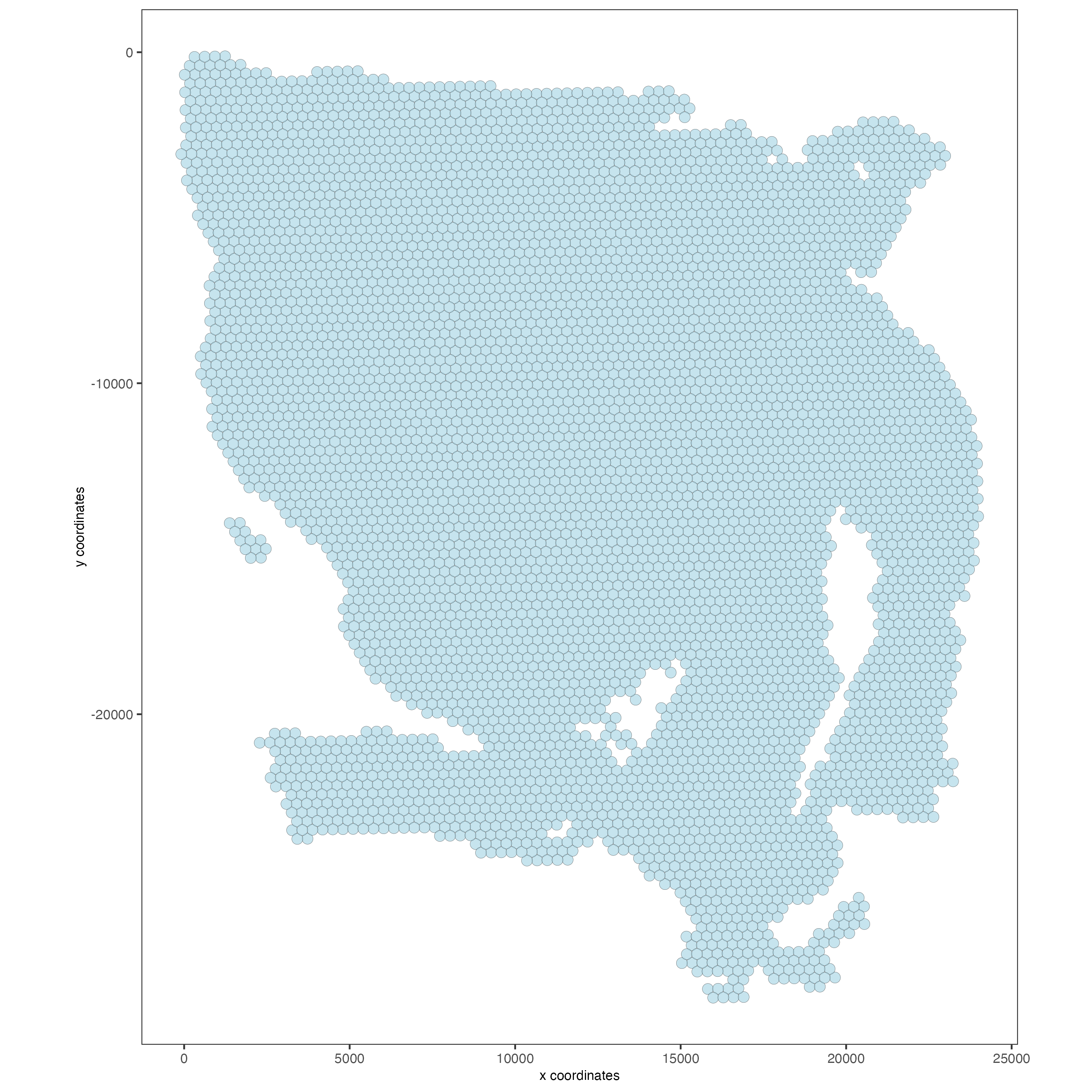
Now that we only have spots from the tissue area, we will remove those spots that contain a very small number of features (genes or proteins), as well as features that are not expressed in enough spots across the sample.
Use the argument min_det_feats_per_cell to set the minimal number of features (genes or proteins) expected per spot. Those spots with less genes or proteins than the provided number will be removed.
Use the argument feat_det_in_min_cells to set the minimal number of spots where each gene or protein should be expressed to be considered in the dataset. Those genes or proteins expressed in less spots than the provided number will be removed.
## RNA
visium <- filterGiotto(gobject = visium,
                       expression_threshold = 1,
                       feat_det_in_min_cells = 50,
                       min_det_feats_per_cell = 1000,
                       expression_values = "raw",
                       verbose = TRUE)

## Protein
visium <- filterGiotto(gobject = visium,
                       spat_unit = "cell",
                       feat_type = "protein",
                       expression_threshold = 1,
                       feat_det_in_min_cells = 50,
                       min_det_feats_per_cell = 1,
                       expression_values = "raw",
                       verbose = TRUE)
5.2 Normalization
Normalize the gene or protein counts by cell, then use the argument scalefactor to set the scale factor to use after library size normalization. The default value is 6000, but you can use a different one.
## RNA
visium <- normalizeGiotto(gobject = visium,
                          scalefactor = 6000,
                          verbose = TRUE)

## Protein
visium <- normalizeGiotto(gobject = visium,
                          spat_unit = "cell",
                          feat_type = "protein",
                          scalefactor = 6000,
                          verbose = TRUE)
5.3 Statistics
Add cell and feature statistics (optional). These values can be used as Quality control, you usually expect to have enough genes or proteins per spot, but the minimal number depends on the experiment design and technology used.
## RNA
visium <- addStatistics(gobject = visium)

### Visualize number of features after processing
spatPlot2D(gobject = visium,
           point_alpha = 0.7,
           cell_color = "nr_feats",
           color_as_factor = FALSE)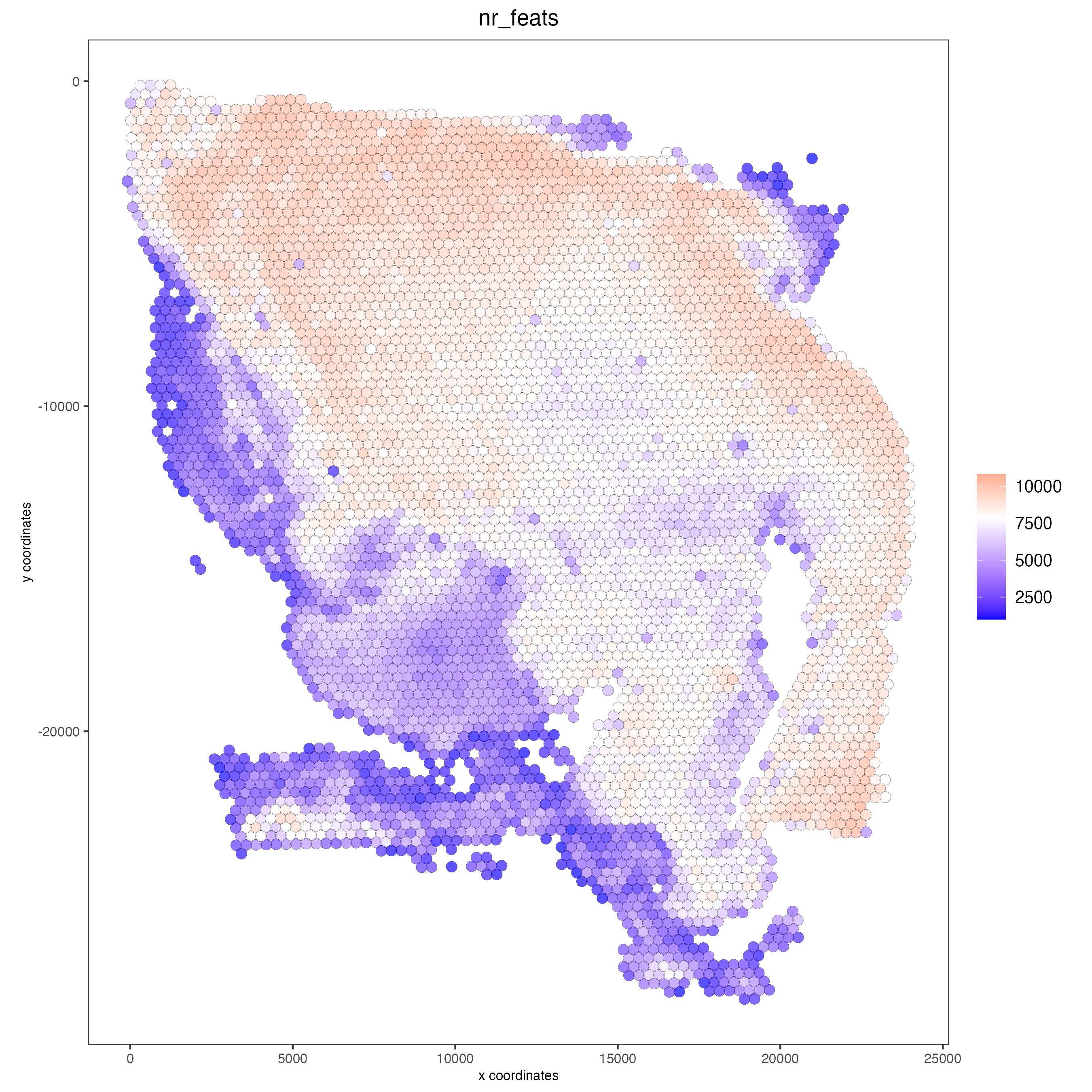
## Protein
visium <- addStatistics(gobject = visium,
                        spat_unit = "cell",
                        feat_type = "protein")

### Visualize number of features after processing
spatPlot2D(gobject = visium,
           spat_unit = "cell",
           feat_type = "protein",
           point_alpha = 0.7,
           cell_color = "nr_feats",
           color_as_factor = FALSE)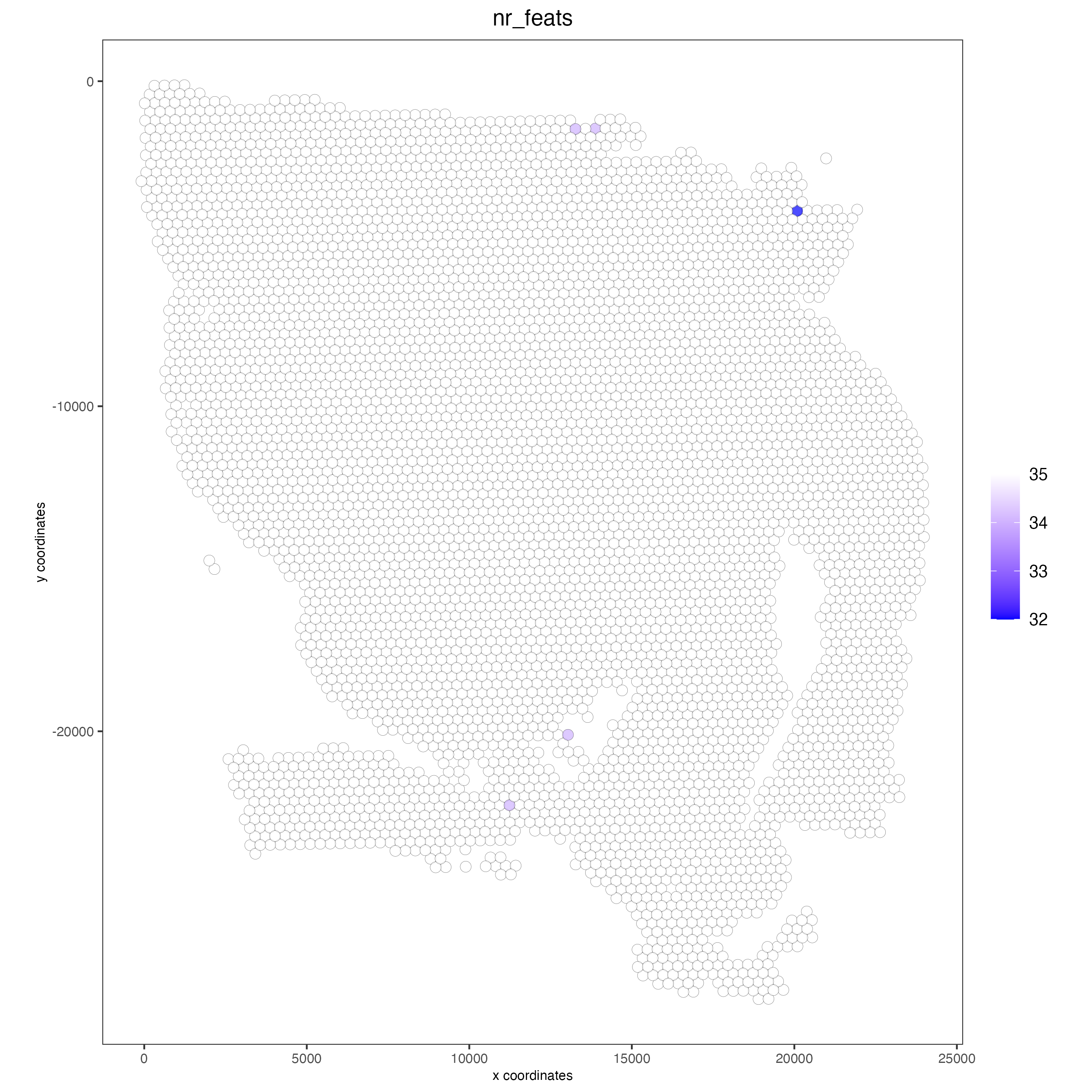
6 Dimension Reduction
6.0.1 Identify highly variable features (HVF)
When having whole transcriptome RNA information, you may want to identify the genes with highest variability and use them for the Principal Components Analysis. This step is not needed for the Protein modality, since the number of proteins is very limited.
## RNA
visium <- calculateHVF(gobject = visium)
6.1 PCA
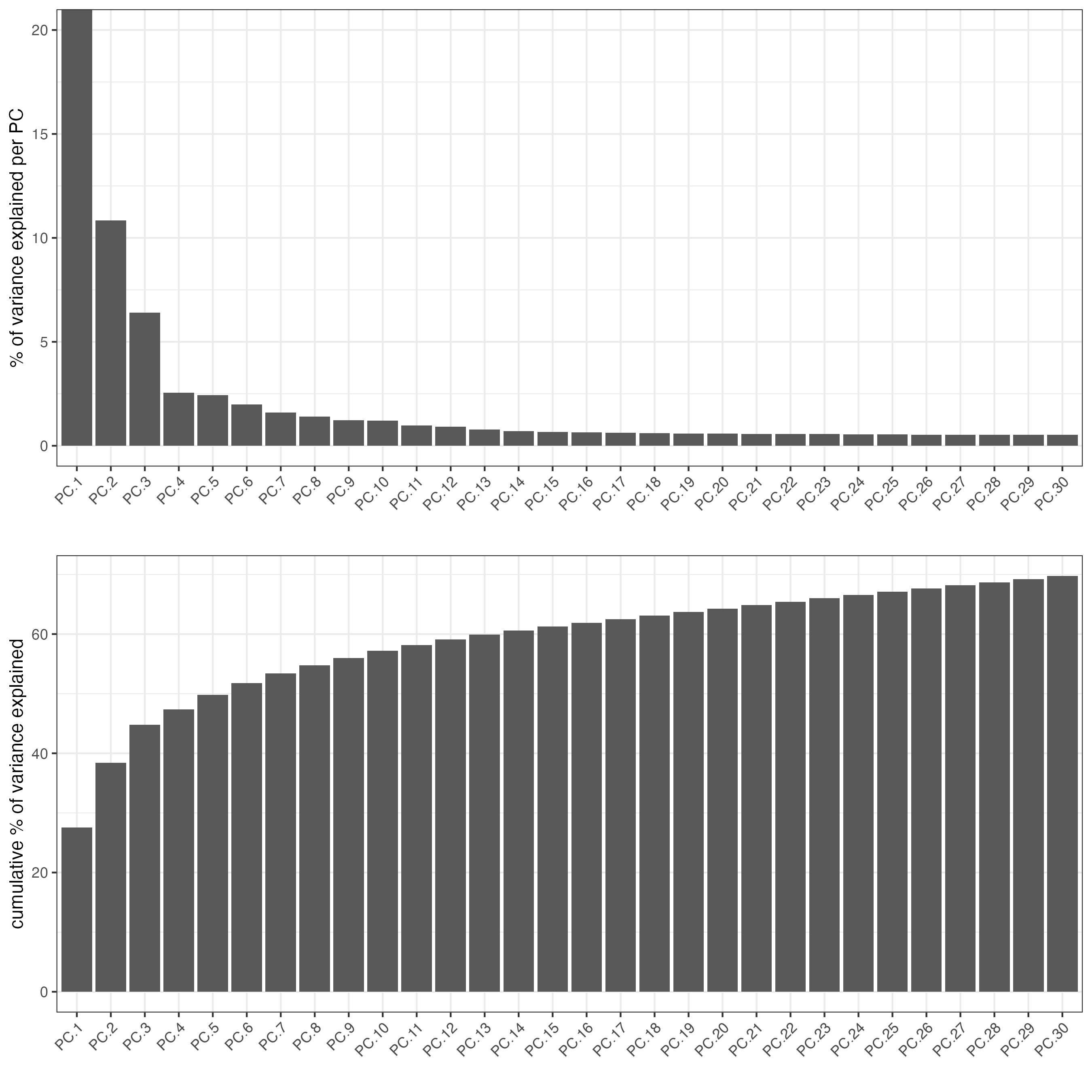
The Principal component Analysis will help to reduce the number of dimensions in the dataset. For the RNA modality, we will use the previously calculated HVFs, but for the protein modality we will use all the proteins available in the dataset.
The screeplot will show how much of the variance of your dataset is explain by each Principal Component. Usually this helps to estimate the number of Principal Components that you should consider for downstream steps.
### Visualize RNA PCA
plotPCA(gobject = visium)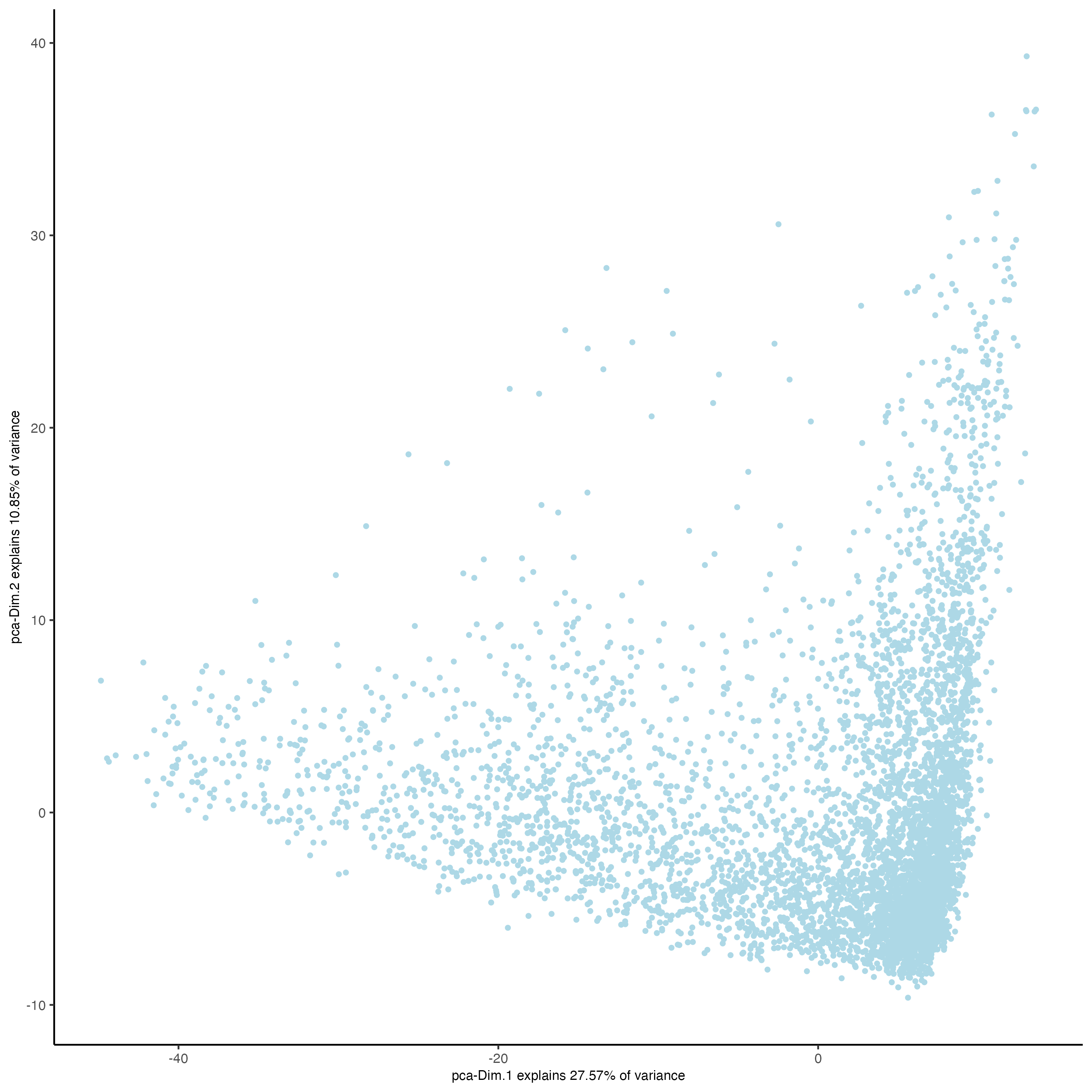
## Protein
visium <- runPCA(gobject = visium,
                 spat_unit = "cell",
                 feat_type = "protein")

screePlot(visium,
          spat_unit = "cell",
          feat_type = "protein",
          ncp = 30)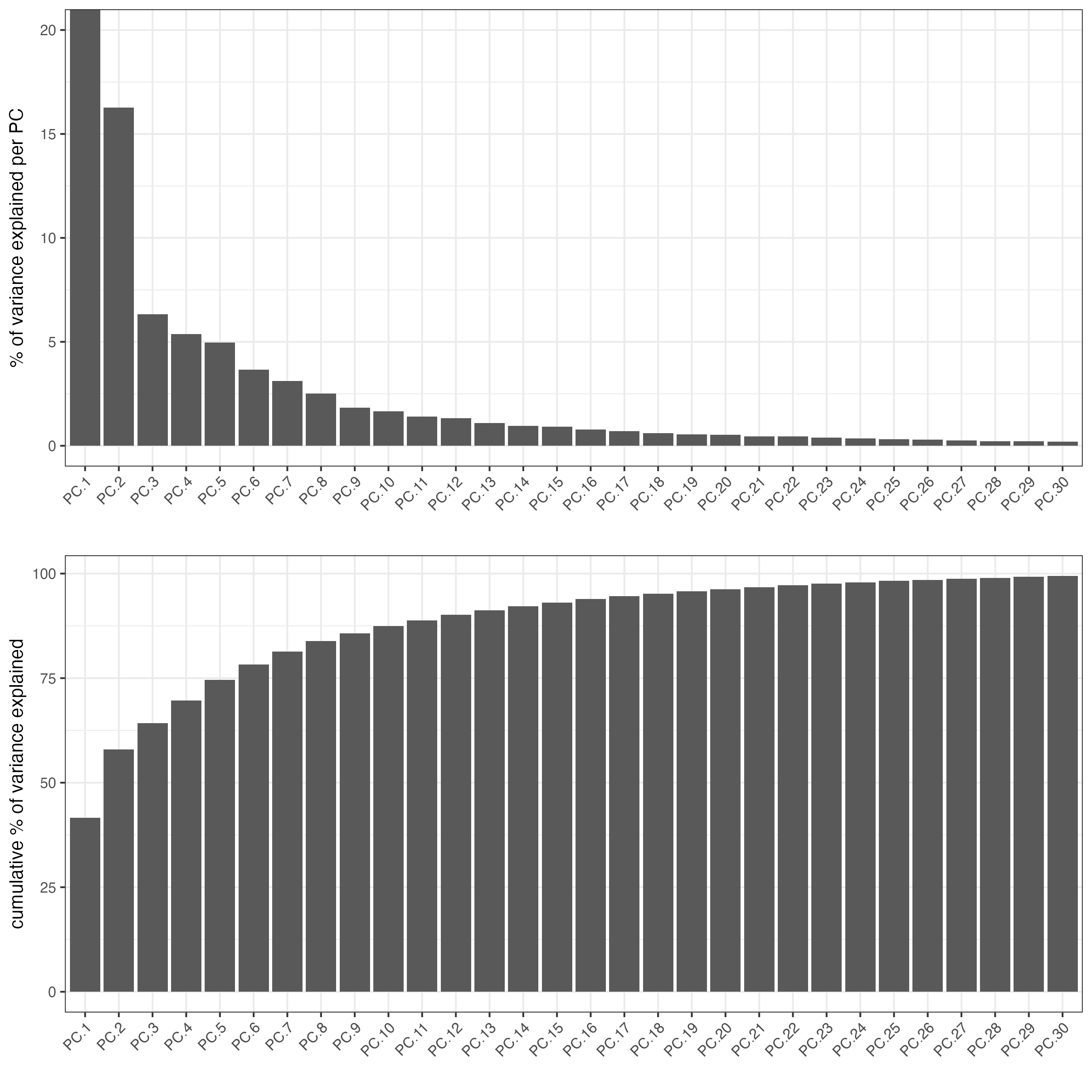
### Visualize Protein PCA
plotPCA(gobject = visium,
        spat_unit = "cell",
        feat_type = "protein")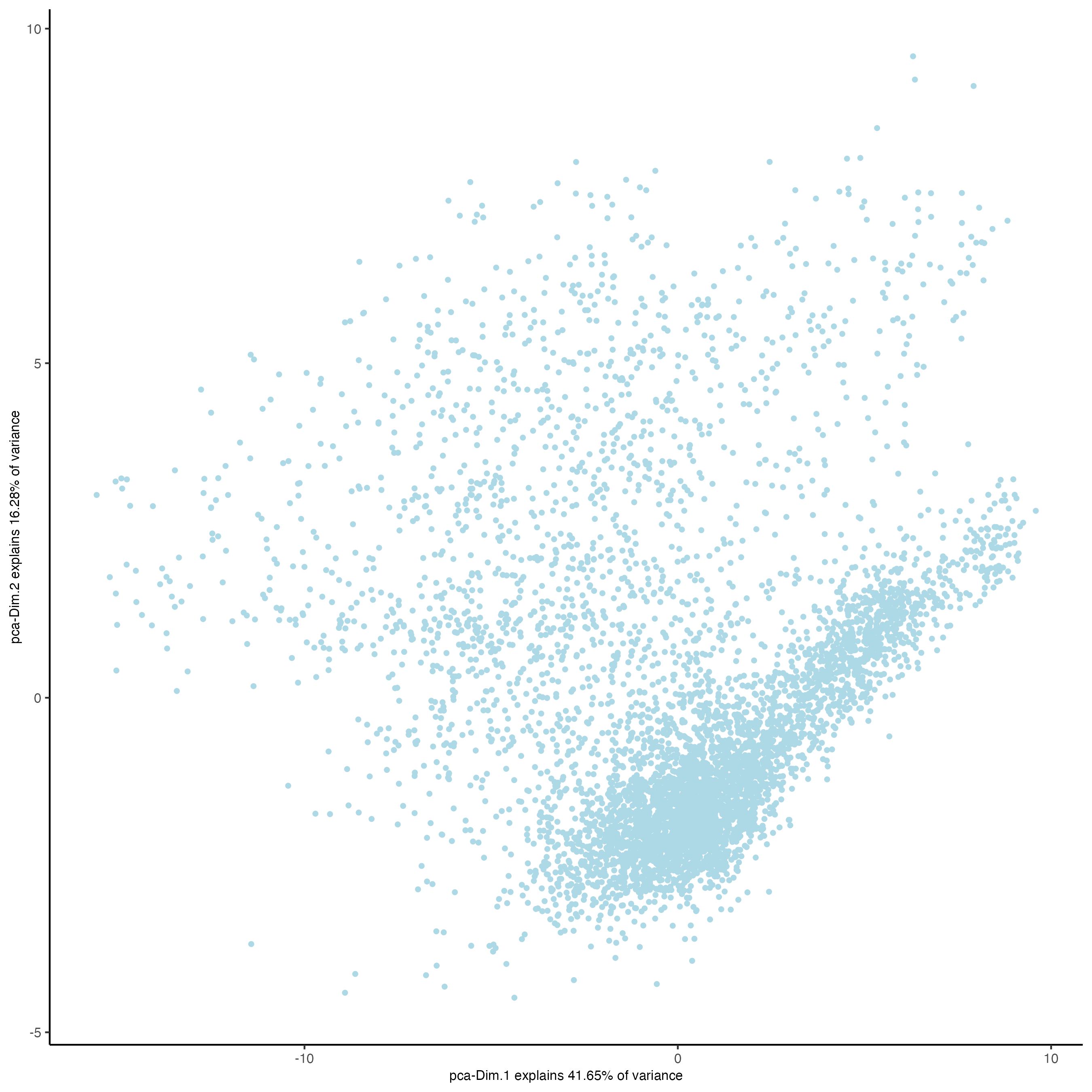
7 Clustering
7.1 UMAP
Unlike PCA, Uniform Manifold Approximation and Projection (UMAP) do not assume linearity. After running the PCA, UMAP allows you to visualize the dataset in 2D.
7.2 sNN network (default)
createNearestNetwork() calculates the nearest neighbors to each spot based on their gene or protein expression. There are two methods available for the calculation, sNN (default) and kNN, You can also use the parameters dimensions_to_use to set how many dimensions from the PCA will be used for the network calculation and how many neighbors (k) to calculate.
## RNA
visium <- createNearestNetwork(gobject = visium,
                               dimensions_to_use = 1:10,
                               k = 30)

## Protein
visium <- createNearestNetwork(gobject = visium,
                               spat_unit = "cell",
                               feat_type = "protein",
                               dimensions_to_use = 1:10,
                               k = 30)
7.3 Leiden clustering
Once you have calculated the spots network, we can cluster the spots based on their similarity. By default, doLeidenCluster uses a resolution of 1, but you can change this value, which usually ranges from 0 (lowest resolution) to 1, but can go further if a higher resolution is needed.
## RNA
visium <- doLeidenCluster(gobject = visium,
                          resolution = 1,
                          n_iterations = 1000)

## Protein
visium <- doLeidenCluster(gobject = visium,
                          spat_unit = "cell",
                          feat_type = "protein",
                          resolution = 1,
                          n_iterations = 1000)

plotUMAP(gobject = visium,
         cell_color = "leiden_clus",
         show_NN_network = TRUE,
         point_size = 2)
Now we can visualize the 2D UMAP and color the spots by Leiden Cluster.
plotUMAP(gobject = visium,
         spat_unit = "cell",
         feat_type = "protein",
         cell_color = "leiden_clus",
         show_NN_network = TRUE,
         point_size = 2)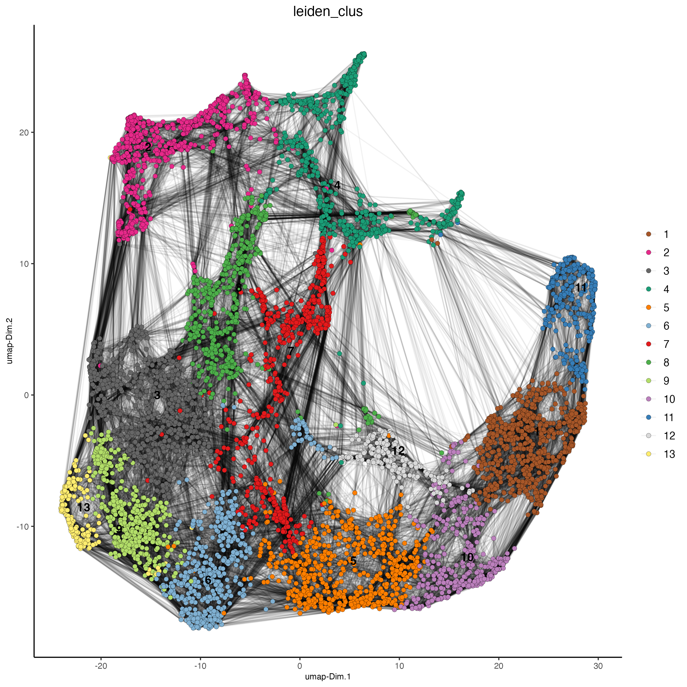
# Visualize spatial plot

## RNA feature
spatPlot2D(gobject = visium,
           show_image = TRUE,
           cell_color = "leiden_clus",
           point_size = 2)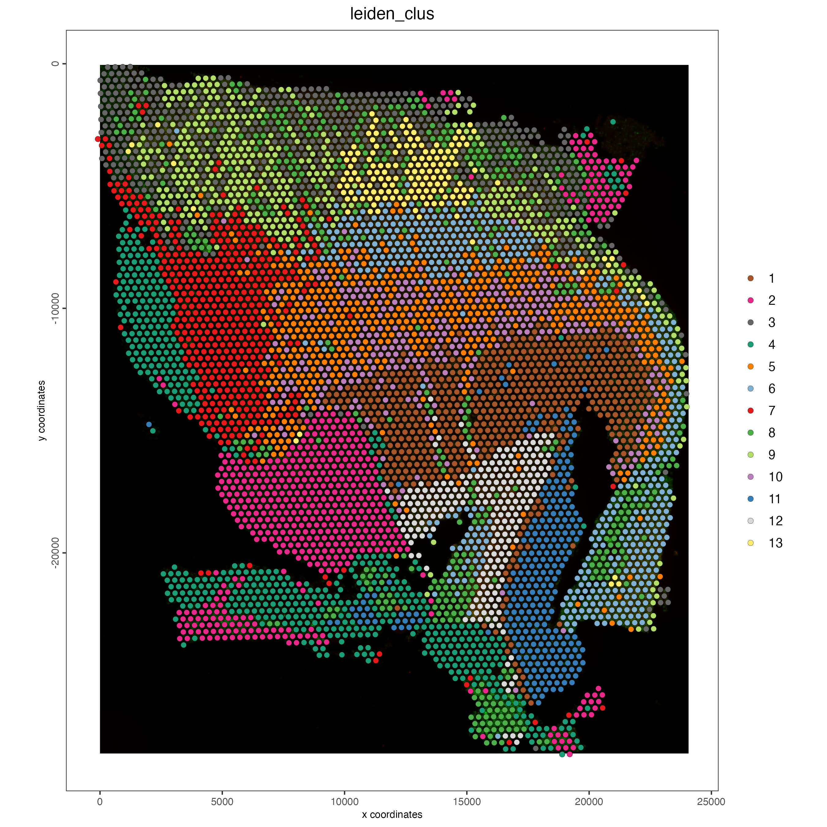
## Protein feature
spatPlot2D(gobject = visium,
           spat_unit = "cell",
           feat_type = "protein",
           show_image = TRUE,
           cell_color = "leiden_clus",
           point_size = 2)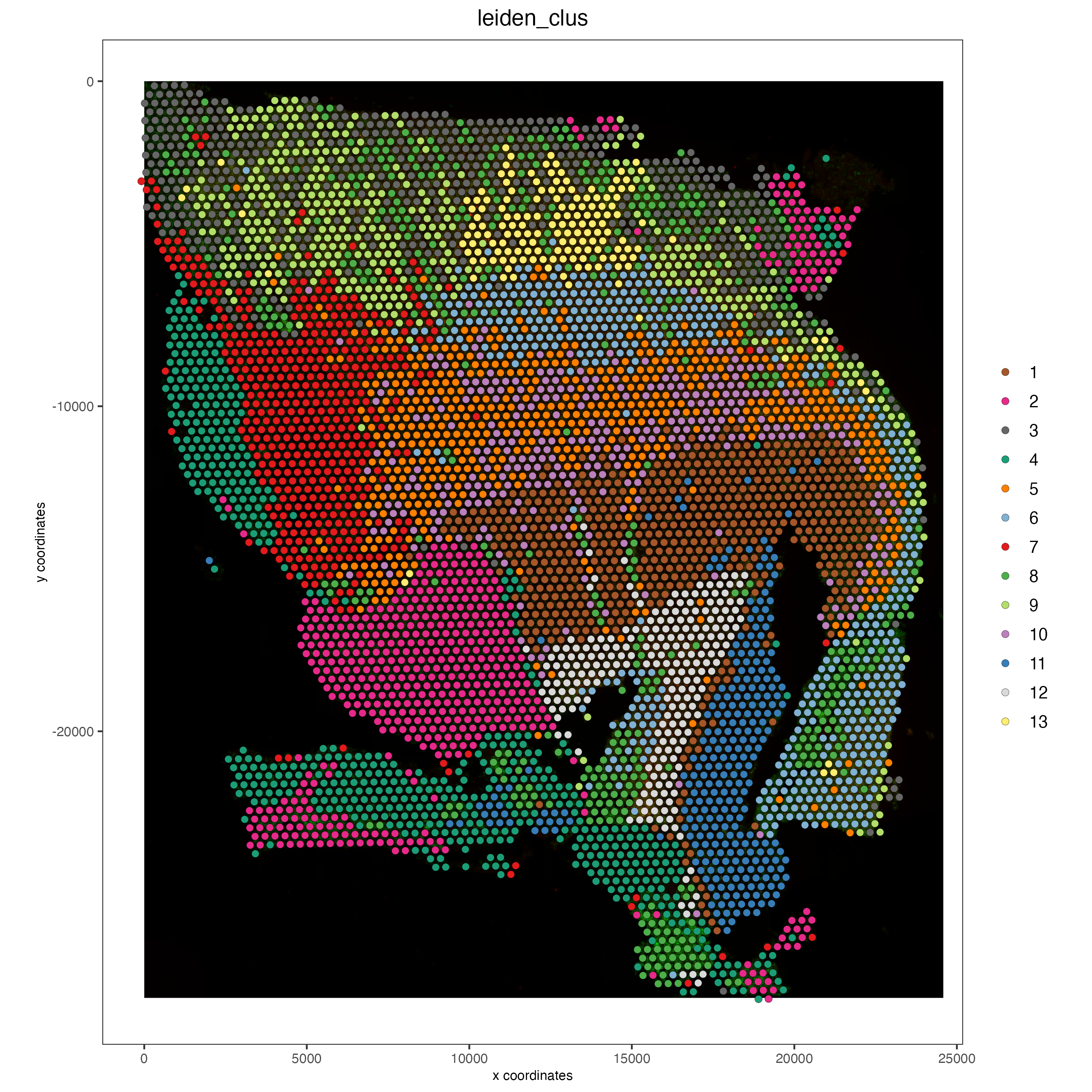
8 Multi-omics integration
The Weighted Nearest Neighbors allows to integrate the modalities acquired from the same sample. WNN will re-calculate the clustering to provide an integrated umap and leiden clustering. For running WNN, the Giotto object must contain the results of running PCA calculation for each modality.
8.1 Calculate kNN
First, we need a nearest network using the kNN method; if you used this method in the clustering step instead of sNN, you can skip this step.
## RNA
visium <- createNearestNetwork(gobject = visium,
                               type = "kNN",
                               dimensions_to_use = 1:10,
                               k = 20)

## Protein
visium <- createNearestNetwork(gobject = visium,
                               spat_unit = "cell",
                               feat_type = "protein",
                               type = "kNN",
                               dimensions_to_use = 1:10,
                               k = 20)
8.2 Run WNN
runWNN will calculate the weight of each modality for each spot and will store the result in the Giotto object under the multiomics slot.
8.3 Run Integrated umap
Using the weights matrix from the previous step, an integrated kNN and UMAP will be calculated, which reflects the integration of the two omics.
visium <- runIntegratedUMAP(visium,
                            feat_types = c("rna", "protein"),
                            force = FALSE)
8.4 Calculate integrated clusters
The final step is calculating the Leiden clusters again, using the integrated information from the previous step. These clusters consider the weight of each modality per spot.
visium <- doLeidenCluster(gobject = visium,
                          spat_unit = "cell",
                          feat_type = "rna",
                          nn_network_to_use = "kNN",
                          network_name = "integrated_kNN",
                          name = "integrated_leiden_clus",
                          resolution = 0.5)

# Visualize integrated umap
plotUMAP(gobject = visium,
         spat_unit = "cell",
         feat_type = "rna",
         cell_color = "integrated_leiden_clus",
         dim_reduction_name = "integrated.umap",
         point_size = 1.5,
         title = "Integrated UMAP using Integrated Leiden clusters",
         axis_title = 12,
         axis_text = 10 )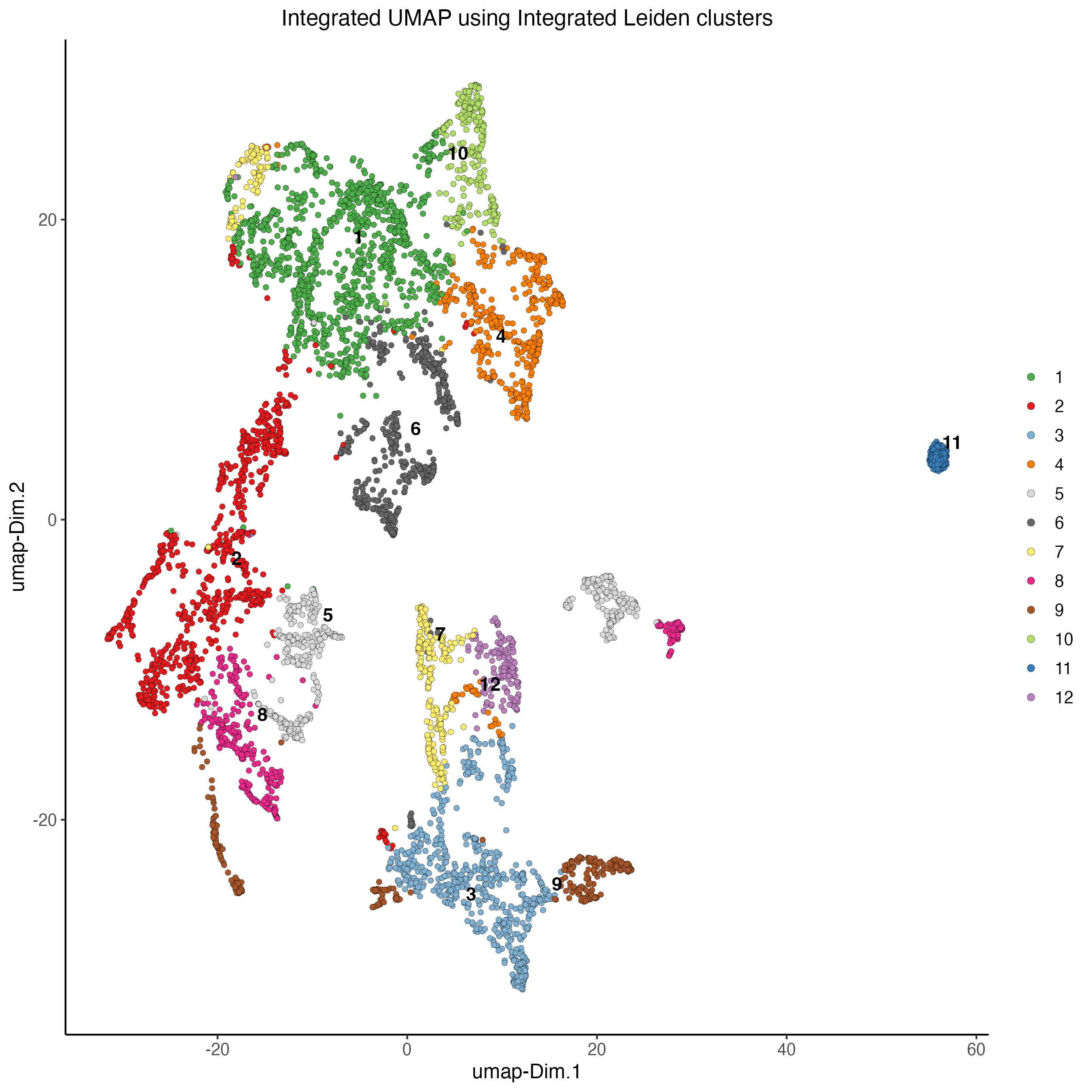
# Visualize spatial plot with integrated clusters
spatPlot2D(visium,
           spat_unit = "cell",
           feat_type = "rna",
           cell_color = "integrated_leiden_clus",
           point_size = 2,
           show_image = FALSE,
           title = "Integrated Leiden clustering")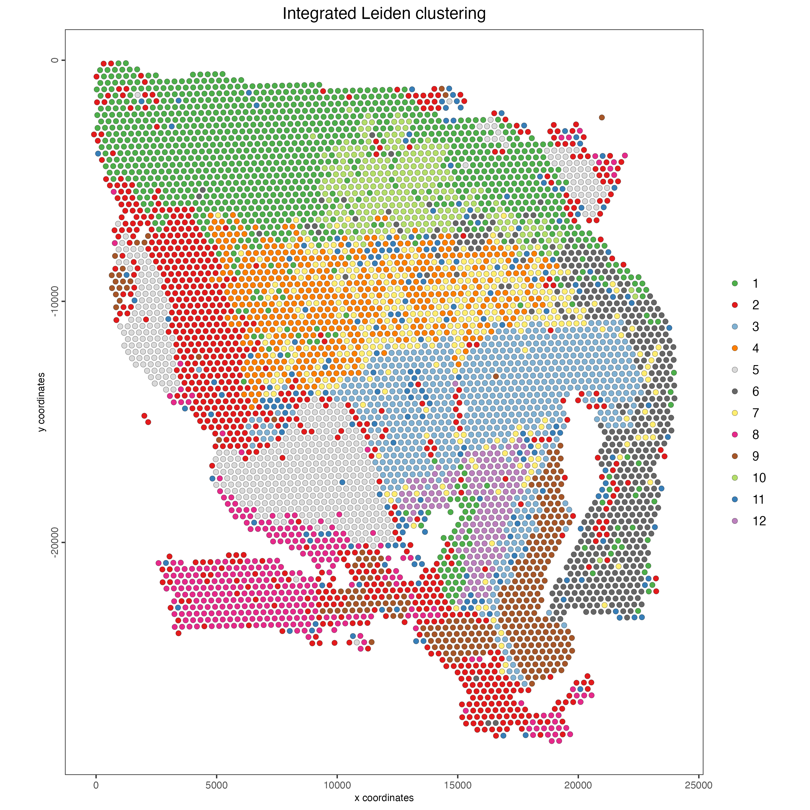
9 Session Info
R version 4.4.1 (2024-06-14)
Platform: x86_64-apple-darwin20
Running under: macOS 15.0

Matrix products: default
BLAS:   /System/Library/Frameworks/Accelerate.framework/Versions/A/Frameworks/vecLib.framework/Versions/A/libBLAS.dylib
LAPACK: /Library/Frameworks/R.framework/Versions/4.4-x86_64/Resources/lib/libRlapack.dylib;  LAPACK version 3.12.0

locale:
[1] en_US.UTF-8/en_US.UTF-8/en_US.UTF-8/C/en_US.UTF-8/en_US.UTF-8

time zone: America/New_York
tzcode source: internal

attached base packages:
[1] stats     graphics  grDevices utils     datasets  methods   base

other attached packages:
[1] Giotto_4.1.3      GiottoClass_0.4.0

loaded via a namespace (and not attached):
  [1] colorRamp2_0.1.0            deldir_2.0-4                rlang_1.1.4
  [4] magrittr_2.0.3              RcppAnnoy_0.0.22            GiottoUtils_0.1.12
  [7] matrixStats_1.4.1           compiler_4.4.1              png_0.1-8
 [10] systemfonts_1.1.0           vctrs_0.6.5                 pkgconfig_2.0.3
 [13] SpatialExperiment_1.14.0    crayon_1.5.3                fastmap_1.2.0
 [16] backports_1.5.0             magick_2.8.5                XVector_0.44.0
 [19] labeling_0.4.3              utf8_1.2.4                  rmarkdown_2.28
 [22] UCSC.utils_1.0.0            ragg_1.3.3                  purrr_1.0.2
 [25] xfun_0.47                   beachmat_2.20.0             zlibbioc_1.50.0
 [28] GenomeInfoDb_1.40.1         jsonlite_1.8.9              DelayedArray_0.30.1
 [31] BiocParallel_1.38.0         terra_1.7-78                irlba_2.3.5.1
 [34] parallel_4.4.1              R6_2.5.1                    RColorBrewer_1.1-3
 [37] reticulate_1.39.0           parallelly_1.38.0           GenomicRanges_1.56.1
 [40] scattermore_1.2             Rcpp_1.0.13                 SummarizedExperiment_1.34.0
 [43] knitr_1.48                  future.apply_1.11.2         R.utils_2.12.3
 [46] IRanges_2.38.1              Matrix_1.7-0                igraph_2.0.3
 [49] tidyselect_1.2.1            rstudioapi_0.16.0           abind_1.4-8
 [52] yaml_2.3.10                 codetools_0.2-20            listenv_0.9.1
 [55] lattice_0.22-6              tibble_3.2.1                Biobase_2.64.0
 [58] withr_3.0.1                 evaluate_1.0.0              future_1.34.0
 [61] pillar_1.9.0                MatrixGenerics_1.16.0       checkmate_2.3.2
 [64] stats4_4.4.1                plotly_4.10.4               generics_0.1.3
 [67] dbscan_1.2-0                sp_2.1-4                    S4Vectors_0.42.1
 [70] ggplot2_3.5.1               munsell_0.5.1               scales_1.3.0
 [73] gtools_3.9.5                globals_0.16.3              glue_1.7.0
 [76] lazyeval_0.2.2              tools_4.4.1                 GiottoVisuals_0.2.5
 [79] data.table_1.16.0           ScaledMatrix_1.12.0         cowplot_1.1.3
 [82] grid_4.4.1                  tidyr_1.3.1                 colorspace_2.1-1
 [85] SingleCellExperiment_1.26.0 GenomeInfoDbData_1.2.12     BiocSingular_1.20.0
 [88] rsvd_1.0.5                  cli_3.6.3                   textshaping_0.4.0
 [91] fansi_1.0.6                 S4Arrays_1.4.1              viridisLite_0.4.2
 [94] dplyr_1.1.4                 uwot_0.2.2                  gtable_0.3.5
 [97] R.methodsS3_1.8.2           digest_0.6.37               BiocGenerics_0.50.0
[100] SparseArray_1.4.8           ggrepel_0.9.6               rjson_0.2.23
[103] htmlwidgets_1.6.4           farver_2.1.2                htmltools_0.5.8.1
[106] R.oo_1.26.0                 lifecycle_1.0.4             httr_1.4.7