1 Dataset explanation
This dataset was deposited in the NeMO database by the Macosko lab under the grant rf1_macosko. It belongs to a mouse brain, processed and sequenced using the Slide-seq technology.
To download the data, run the following code:
# Provide path to the data folder
data_path <- "/path/to/data/"- Get the expression data
download.file(url = "https://data.nemoarchive.org/biccn/grant/rf1_macosko/macosko/spatial_transcriptome/cellgroup/Slide-seq/mouse/processed/counts/2020-12-19_Puck_201112_26.matched.digital_expression.mex.tar.gz",
destfile = file.path(data_path, "2020-12-19_Puck_201112_26.matched.digital_expression.mex.tar.gz"))- Get the spatial coordinates
download.file(url = "https://data.nemoarchive.org/biccn/grant/rf1_macosko/macosko/spatial_transcriptome/cellgroup/Slide-seq/mouse/processed/other/2020-12-19_Puck_201112_26.BeadLocationsForR.csv.tar",
destfile = file.path(data_path, "2020-12-19_Puck_201112_26.BeadLocationsForR.csv.tar"))- Untar the expression files running:
2 Start Giotto
# Ensure Giotto Suite is installed
if(!"Giotto" %in% installed.packages()) {
  pak::pkg_install("drieslab/Giotto")
}

# Ensure the Python environment for Giotto has been installed
genv_exists <- Giotto::checkGiottoEnvironment()

if(!genv_exists){
  # The following command need only be run once to install the Giotto environment
  Giotto::installGiottoEnvironment()
}
library(Giotto)

# 1. set results directory
results_folder <- "/path/to/results/"

# 2. set giotto python path
# set python path to your preferred python version path
# set python path to NULL if you want to automatically install (only the 1st time) and use the giotto miniconda environment
python_path <- NULL

# 3. create giotto instructions
instructions <- createGiottoInstructions(save_dir = results_folder,
                                         save_plot = TRUE,
                                         show_plot = FALSE,
                                         return_plot = FALSE,
                                         python_path = python_path)
3 Create Giotto object
- Read the expression files and create the expression matrix.
expression_matrix <- get10Xmatrix(file.path(data_path, "2020-12-19_Puck_201112_26.matched.digital_expression"))- Read the spatial coordinates file and filter the cell IDs.
spatial_locs <- data.table::fread(file.path(data_path, "2020-12-19_Puck_201112_26.BeadLocationsForR.csv.tar"))

spatial_locs <- spatial_locs[spatial_locs$barcodes %in% colnames(expression_matrix),]- Create the Giotto object
giotto_object <- createGiottoObject(
  expression = expression_matrix,
  spatial_locs = spatial_locs,
  instructions = instructions
)- Visualize the dataset
spatPlot2D(giotto_object,
           point_size = 2)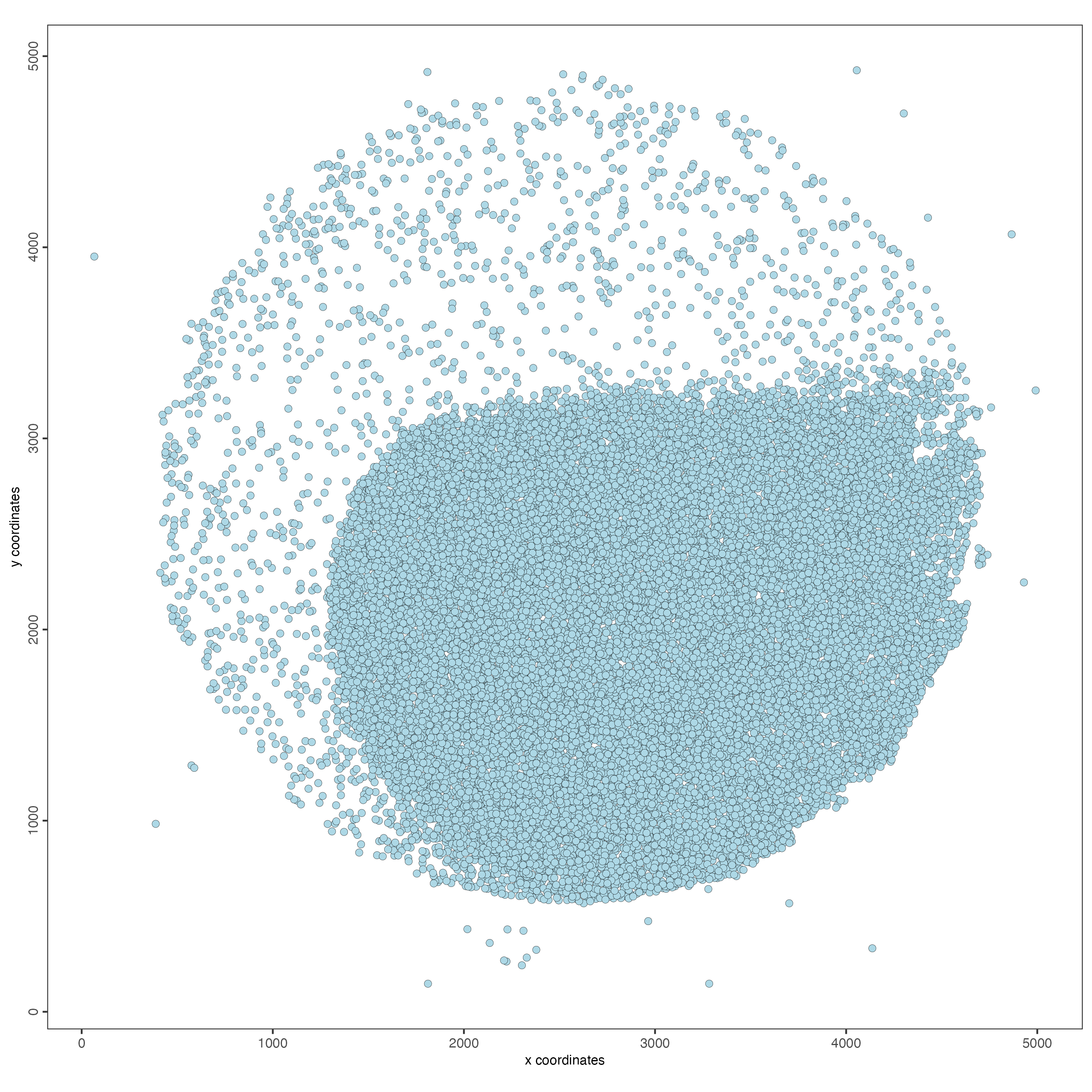
4 Processing
4.1 Filtering
giotto_object <- filterGiotto(giotto_object,
                              min_det_feats_per_cell = 10,
                              feat_det_in_min_cells = 10)
4.2 Normalization
giotto_object <- normalizeGiotto(giotto_object)4.3 Add statistics
giotto_object <- addStatistics(giotto_object)

spatPlot2D(giotto_object,
           cell_color = "nr_feats",
           color_as_factor = FALSE,
           point_size = 1)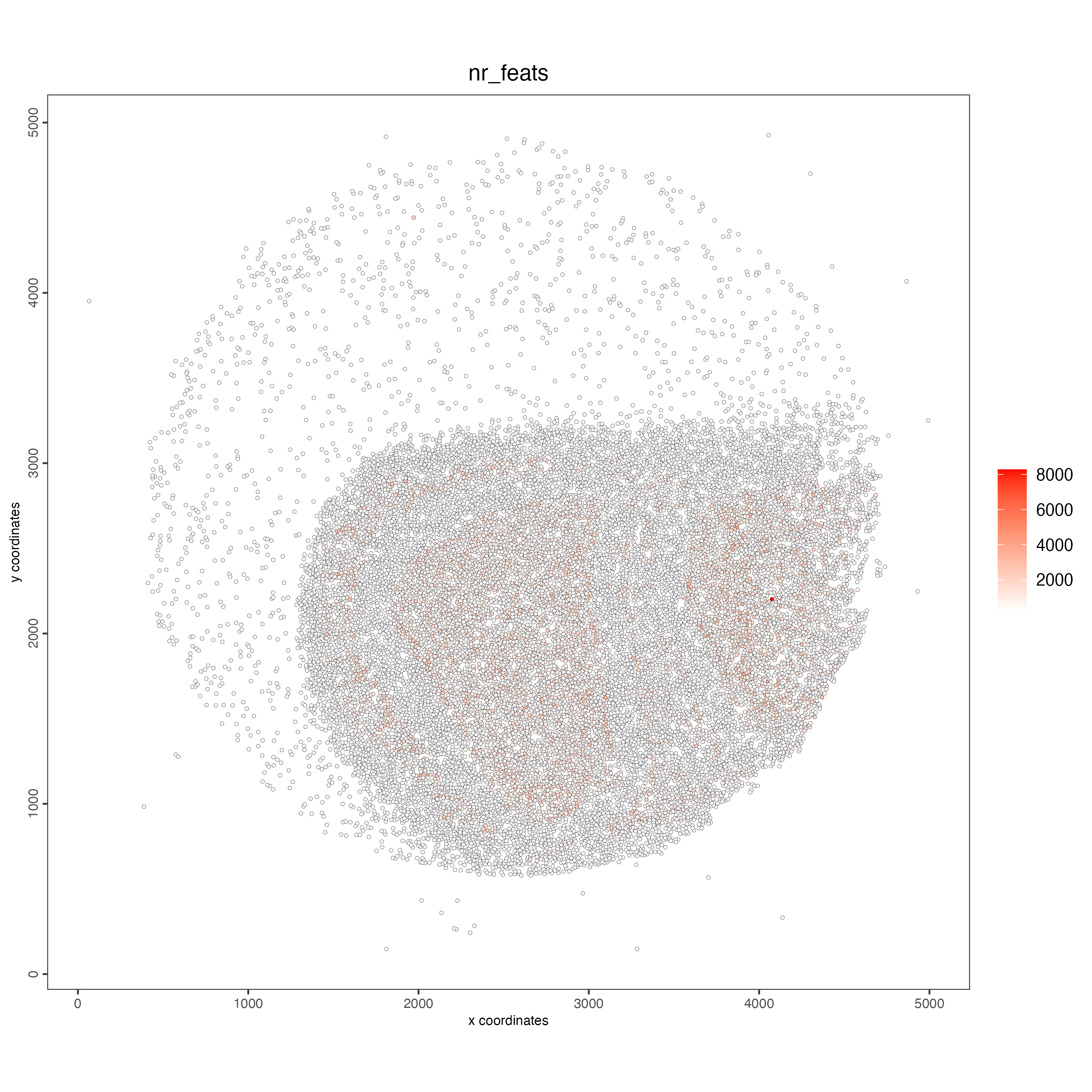
4.5 Clustering
giotto_object <- runUMAP(giotto_object,
                         dimensions_to_use = 1:10)

giotto_object <- createNearestNetwork(giotto_object)

giotto_object <- doLeidenCluster(giotto_object,
                                 resolution = 1)
4.6 Plot
plotPCA(giotto_object,
        cell_color = "leiden_clus",
        point_size = 1)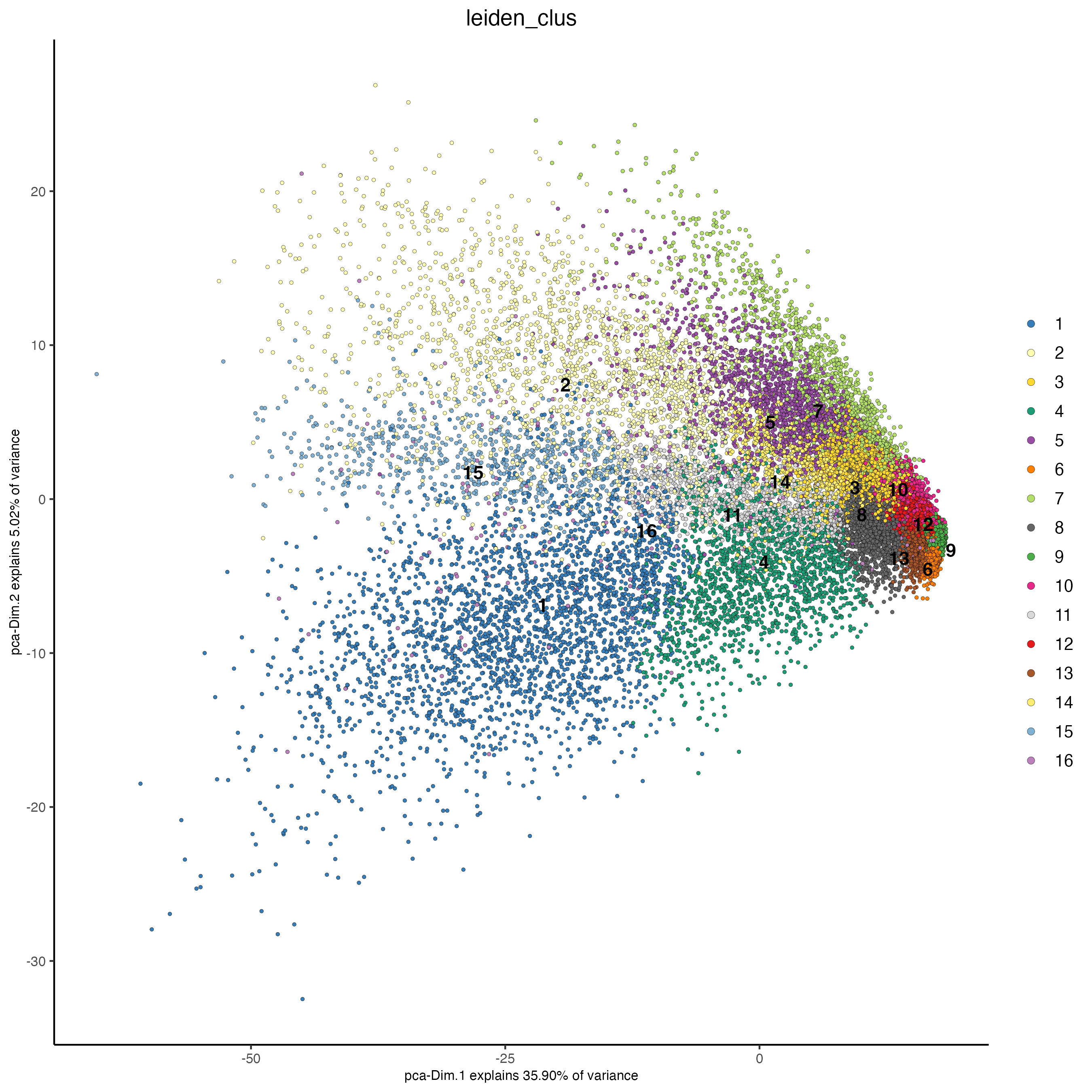
plotUMAP(giotto_object,
         cell_color = "leiden_clus",
         point_size = 1)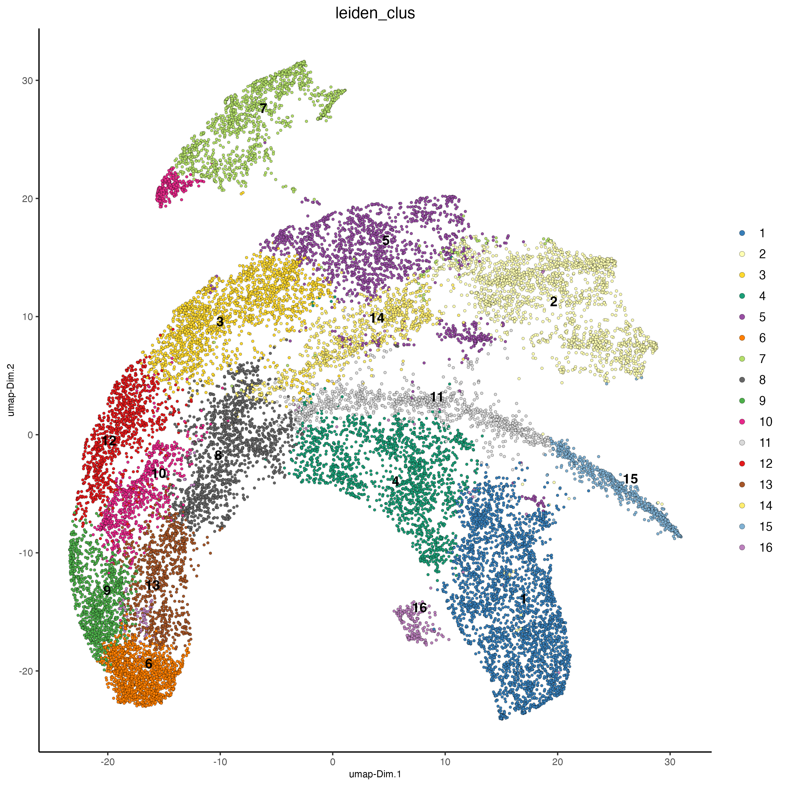
spatPlot2D(giotto_object,
           cell_color = "leiden_clus",
           point_size = 1)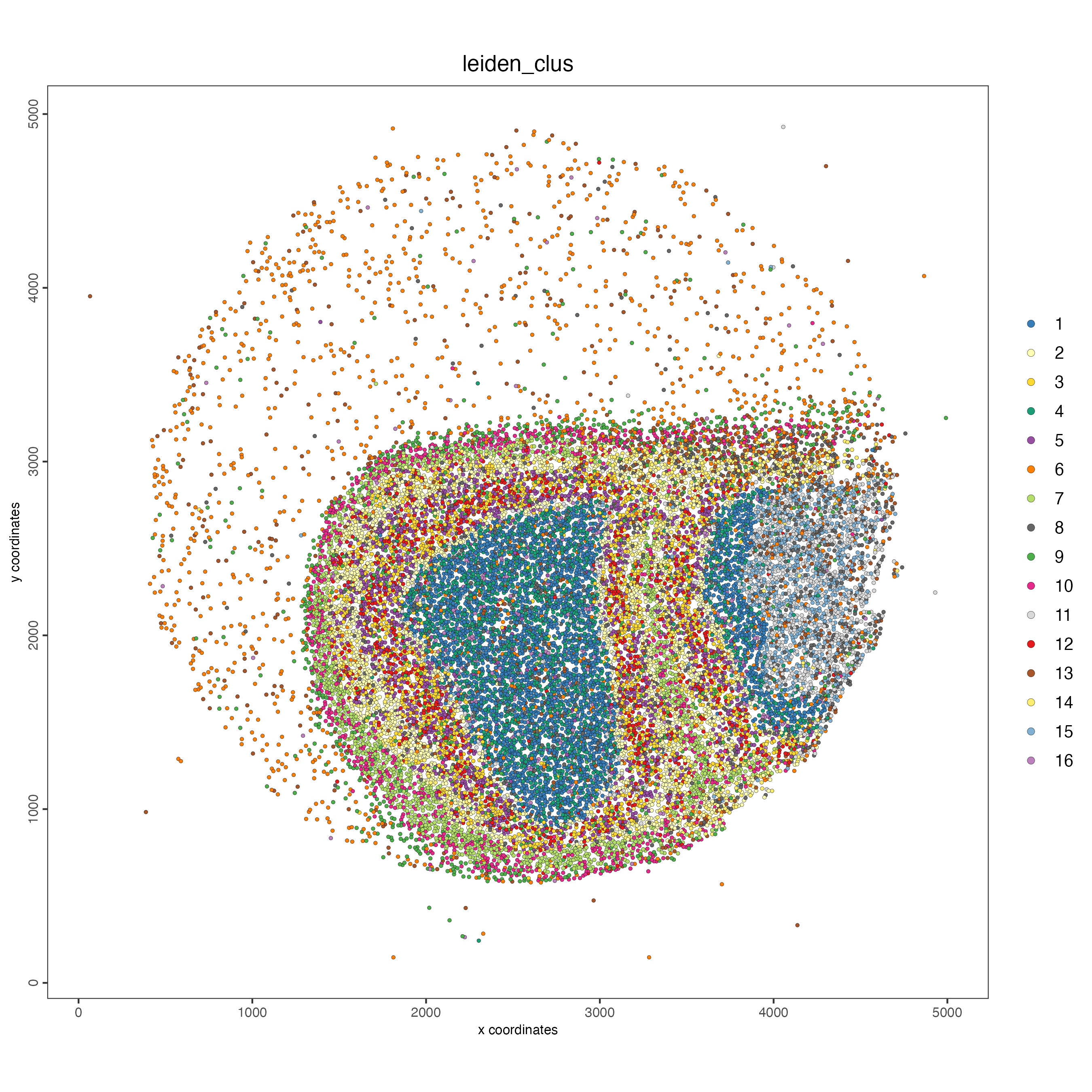
5 Session info
R version 4.4.0 (2024-04-24)
Platform: x86_64-apple-darwin20
Running under: macOS Sonoma 14.6.1

Matrix products: default
BLAS:   /System/Library/Frameworks/Accelerate.framework/Versions/A/Frameworks/vecLib.framework/Versions/A/libBLAS.dylib
LAPACK: /Library/Frameworks/R.framework/Versions/4.4-x86_64/Resources/lib/libRlapack.dylib;  LAPACK version 3.12.0

locale:
[1] en_US.UTF-8/en_US.UTF-8/en_US.UTF-8/C/en_US.UTF-8/en_US.UTF-8

time zone: America/New_York
tzcode source: internal

attached base packages:
[1] stats     graphics  grDevices utils     datasets  methods   base

other attached packages:
[1] Giotto_4.1.1      GiottoClass_0.3.5

loaded via a namespace (and not attached):
  [1] colorRamp2_0.1.0            deldir_2.0-4
  [3] rlang_1.1.4                 magrittr_2.0.3
  [5] RcppAnnoy_0.0.22            GiottoUtils_0.1.11
  [7] matrixStats_1.3.0           compiler_4.4.0
  [9] png_0.1-8                   systemfonts_1.1.0
 [11] vctrs_0.6.5                 reshape2_1.4.4
 [13] stringr_1.5.1               pkgconfig_2.0.3
 [15] SpatialExperiment_1.14.0    crayon_1.5.3
 [17] fastmap_1.2.0               backports_1.5.0
 [19] magick_2.8.4                XVector_0.44.0
 [21] labeling_0.4.3              utf8_1.2.4
 [23] rmarkdown_2.28              UCSC.utils_1.0.0
 [25] ragg_1.3.2                  purrr_1.0.2
 [27] xfun_0.47                   beachmat_2.20.0
 [29] zlibbioc_1.50.0             GenomeInfoDb_1.40.1
 [31] jsonlite_1.8.8              DelayedArray_0.30.1
 [33] BiocParallel_1.38.0         terra_1.7-78
 [35] irlba_2.3.5.1               parallel_4.4.0
 [37] R6_2.5.1                    stringi_1.8.4
 [39] RColorBrewer_1.1-3          reticulate_1.38.0
 [41] GenomicRanges_1.56.1        scattermore_1.2
 [43] Rcpp_1.0.13                 SummarizedExperiment_1.34.0
 [45] knitr_1.48                  R.utils_2.12.3
 [47] IRanges_2.38.1              Matrix_1.7-0
 [49] igraph_2.0.3                tidyselect_1.2.1
 [51] rstudioapi_0.16.0           abind_1.4-5
 [53] yaml_2.3.10                 codetools_0.2-20
 [55] lattice_0.22-6              tibble_3.2.1
 [57] plyr_1.8.9                  Biobase_2.64.0
 [59] withr_3.0.1                 evaluate_0.24.0
 [61] pillar_1.9.0                MatrixGenerics_1.16.0
 [63] checkmate_2.3.2             stats4_4.4.0
 [65] plotly_4.10.4               generics_0.1.3
 [67] dbscan_1.2-0                sp_2.1-4
 [69] S4Vectors_0.42.1            ggplot2_3.5.1
 [71] munsell_0.5.1               scales_1.3.0
 [73] gtools_3.9.5                glue_1.7.0
 [75] lazyeval_0.2.2              tools_4.4.0
 [77] GiottoVisuals_0.2.5         data.table_1.15.4
 [79] ScaledMatrix_1.12.0         cowplot_1.1.3
 [81] grid_4.4.0                  tidyr_1.3.1
 [83] colorspace_2.1-1            SingleCellExperiment_1.26.0
 [85] GenomeInfoDbData_1.2.12     BiocSingular_1.20.0
 [87] rsvd_1.0.5                  cli_3.6.3
 [89] textshaping_0.4.0           fansi_1.0.6
 [91] S4Arrays_1.4.1              viridisLite_0.4.2
 [93] dplyr_1.1.4                 uwot_0.2.2
 [95] gtable_0.3.5                R.methodsS3_1.8.2
 [97] digest_0.6.37               BiocGenerics_0.50.0
 [99] SparseArray_1.4.8           ggrepel_0.9.5
[101] rjson_0.2.22                htmlwidgets_1.6.4
[103] farver_2.1.2                htmltools_0.5.8.1
[105] R.oo_1.26.0                 lifecycle_1.0.4
[107] httr_1.4.7