1 Start Giotto
# Ensure Giotto Suite is installed.
if(!"Giotto" %in% installed.packages()) {
  pak::pkg_install("drieslab/Giotto")
}

# Ensure GiottoData, a small, helper module for tutorials, is installed.
if(!"GiottoData" %in% installed.packages()) {
  pak::pkg_install("drieslab/GiottoData")
}

# Ensure the Python environment for Giotto has been installed.
genv_exists <- Giotto::checkGiottoEnvironment()
if(!genv_exists){
  # The following command need only be run once to install the Giotto environment.
  Giotto::installGiottoEnvironment()
}
2 Load the Giotto object
A small seqFISH data is available through the giottoData package.
# download data
seqfish_mini <- loadGiottoMini("seqfish",
                               python_path = NULL)
2.1 Set Giotto instructions (optional)
How to work with Giotto instructions that are part of your Giotto object:
- Show the instructions associated with your Giotto object with showGiottoInstructions()
- Change one or more instructions with changeGiottoInstructions()
- Replace all instructions at once with replaceGiottoInstructions()
- Read or get a specific Giotto instruction with readGiottoInstructions()
# show instructions associated with giotto object (seqfish_mini)
showGiottoInstructions(seqfish_mini)

# Change one or more instructions
# to automatically save figures in save_dir, set save_plot to TRUE
results_folder <- "/path/to/results/"

seqfish_mini <- changeGiottoInstructions(seqfish_mini,
                                         params = c("save_dir", "save_plot", "show_plot"),
                                         new_values = c(results_folder,TRUE, TRUE))
3 Processing steps
- Filter genes and cells based on detection frequencies.
- Normalize expression matrix (log transformation, scaling factor and/or z-scores)
- Add cell and gene statistics (optional)
- Adjust expression matrix for technical covariates or batches (optional). These results will be stored in the custom slot.
seqfish_mini <- filterGiotto(gobject = seqfish_mini,
                             expression_threshold = 0.5,
                             feat_det_in_min_cells = 20,
                             min_det_feats_per_cell = 0)

seqfish_mini <- normalizeGiotto(gobject = seqfish_mini,
                                scalefactor = 6000,
                                verbose = TRUE)

seqfish_mini <- addStatistics(gobject = seqfish_mini)

seqfish_mini <- adjustGiottoMatrix(gobject = seqfish_mini,
                                   expression_values = "normalized",
                                   covariate_columns = c("nr_feats", "total_expr"))
4 Dimension reduction
- Identify highly variable features (HVF)
seqfish_mini <- calculateHVF(gobject = seqfish_mini)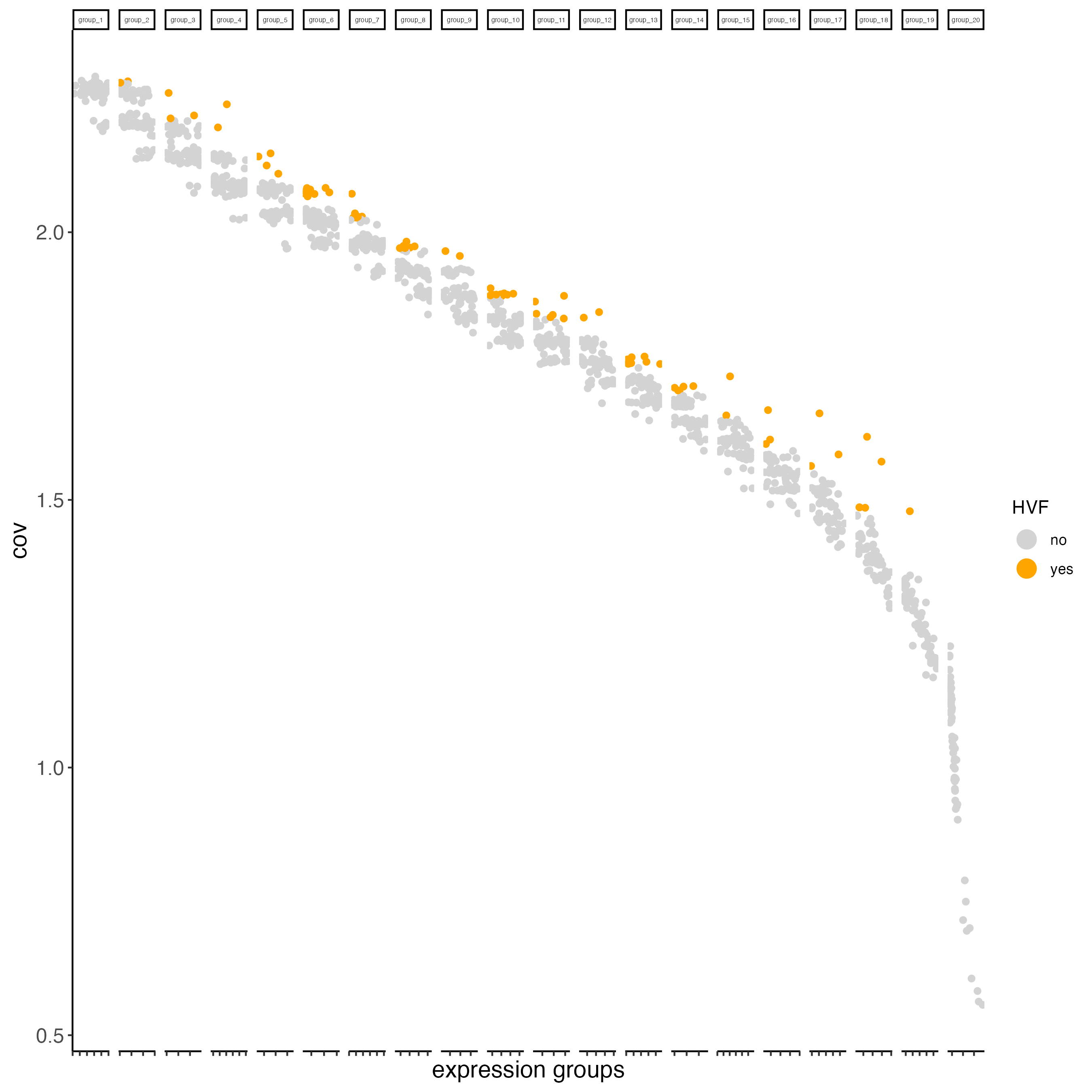
- Perform PCA
- Identify number of significant principal components (PCs)
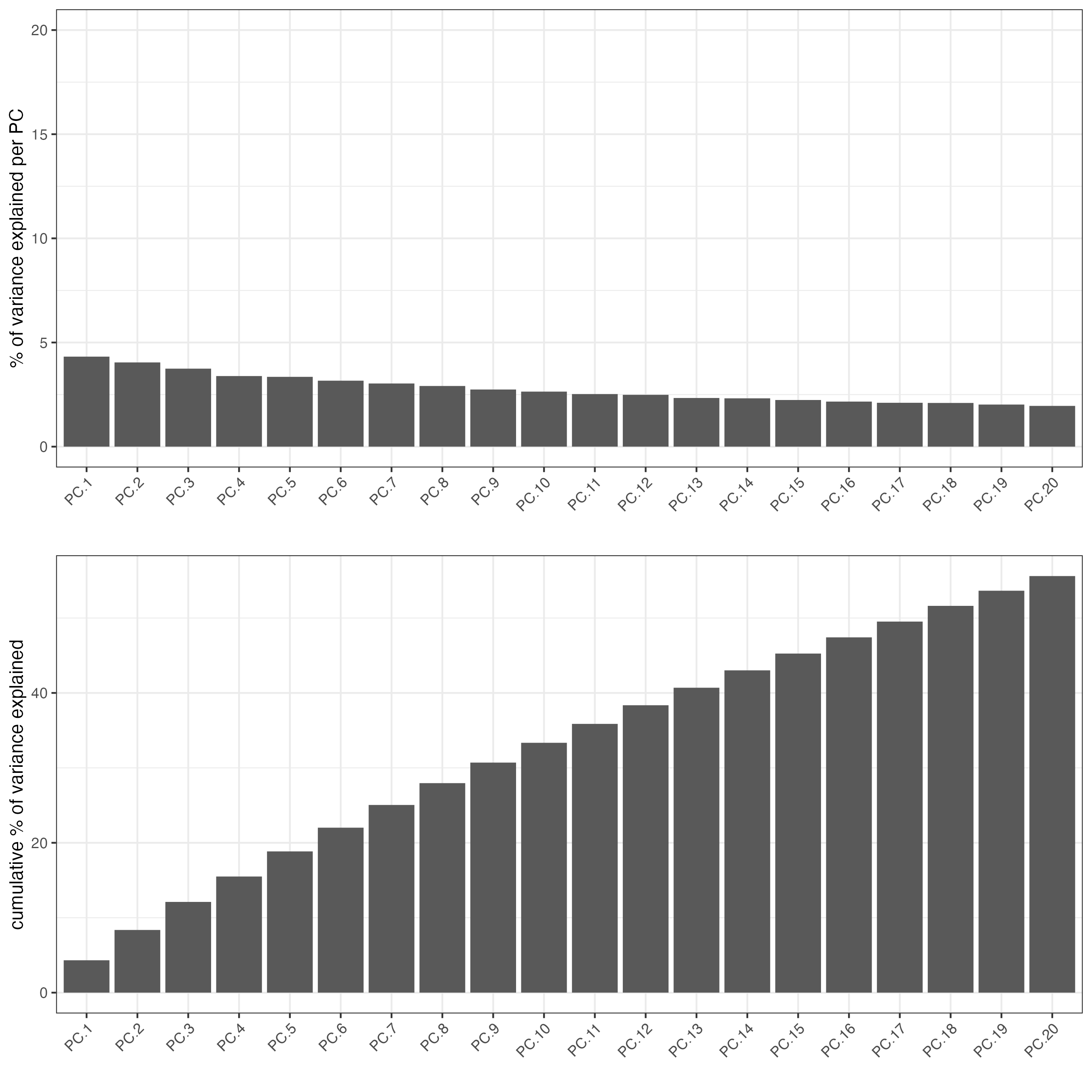
plotPCA(seqfish_mini)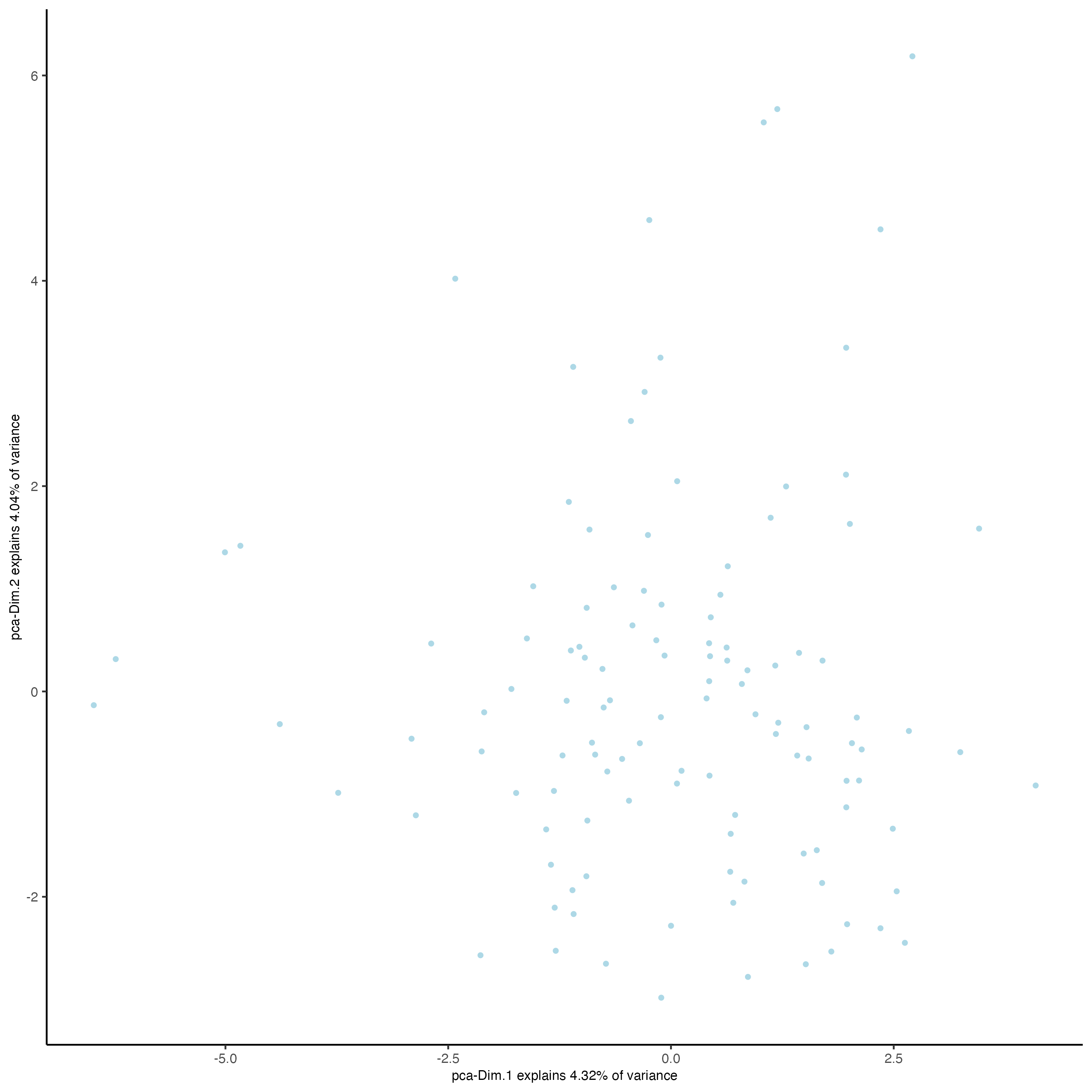
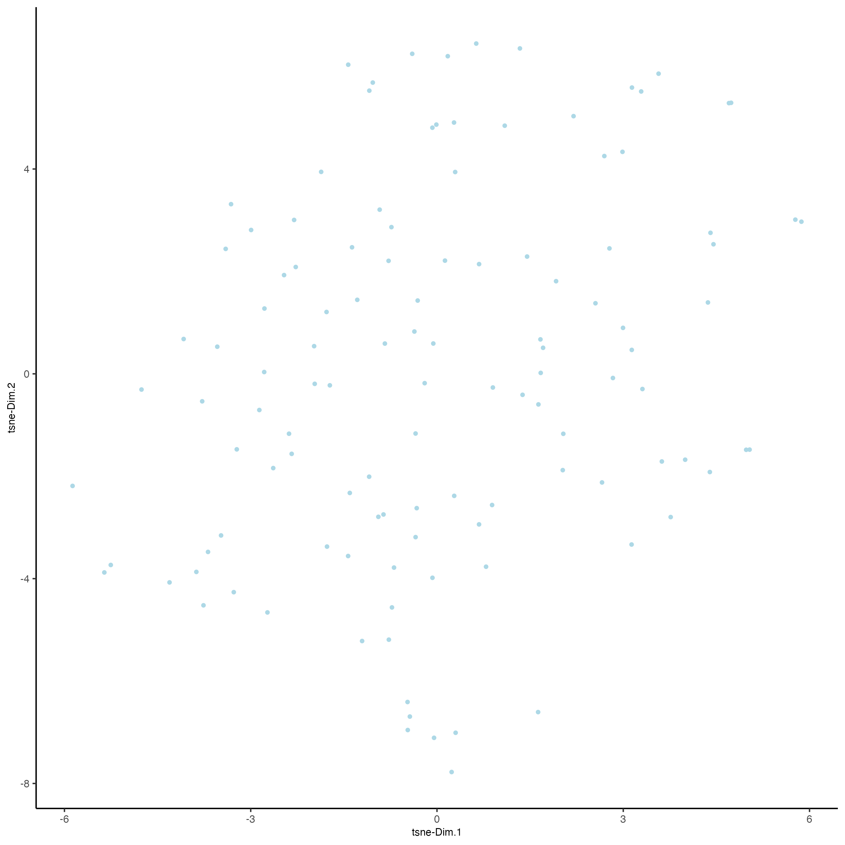
- Run UMAP and/or t-SNE on PCs (or directly on matrix)
seqfish_mini <- runUMAP(seqfish_mini,
                        dimensions_to_use = 1:5,
                        n_threads = 2)

plotUMAP(gobject = seqfish_mini)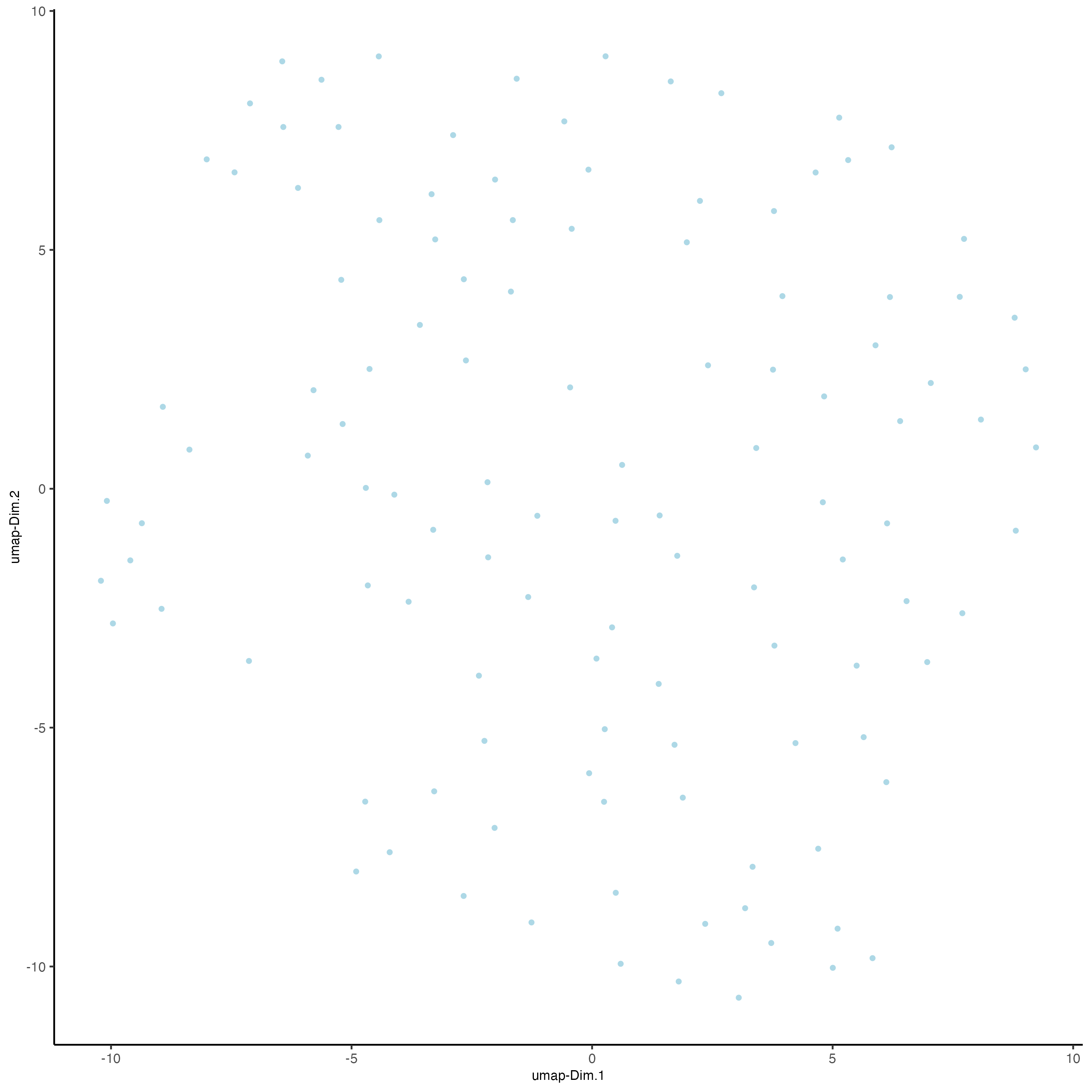
5 Clustering
- Create a shared (default) nearest network in PCA space (or directly on matrix)
- Cluster on nearest network with Leiden or Louvain (k-means and hclust are alternatives)
seqfish_mini <- createNearestNetwork(gobject = seqfish_mini,
                                     dimensions_to_use = 1:5,
                                     k = 5)

seqfish_mini <- doLeidenCluster(gobject = seqfish_mini,
                                resolution = 0.4,
                                n_iterations = 1000)

# visualize UMAP cluster results
plotUMAP(gobject = seqfish_mini,
         cell_color = "leiden_clus",
         show_NN_network = TRUE,
         point_size = 2.5)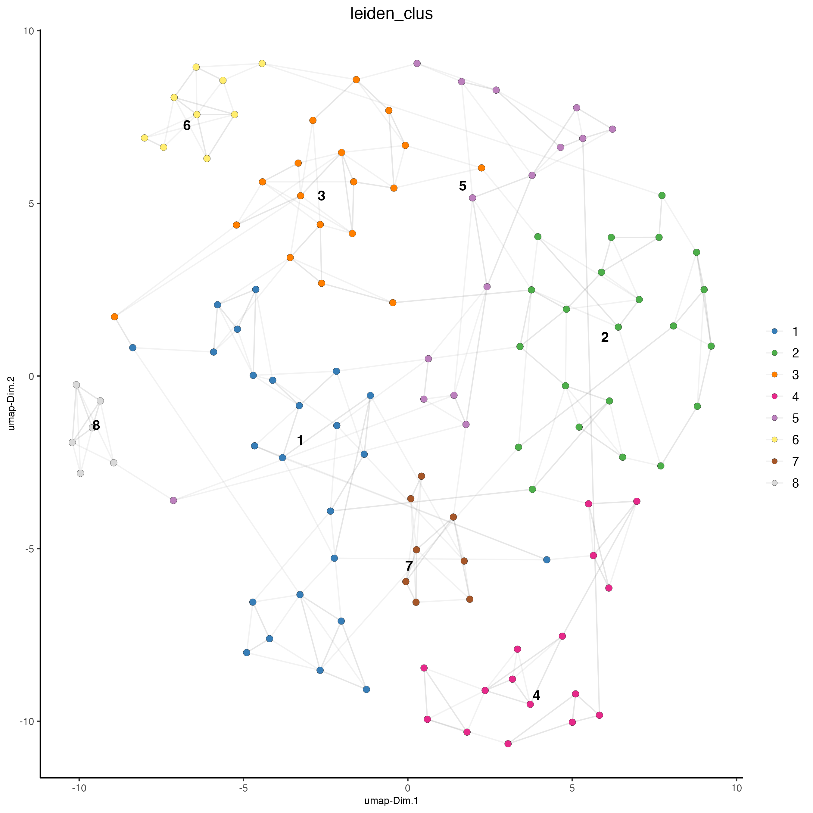
# visualize UMAP and spatial results
spatDimPlot(gobject = seqfish_mini,
            cell_color = "leiden_clus",
            spat_point_shape = "voronoi")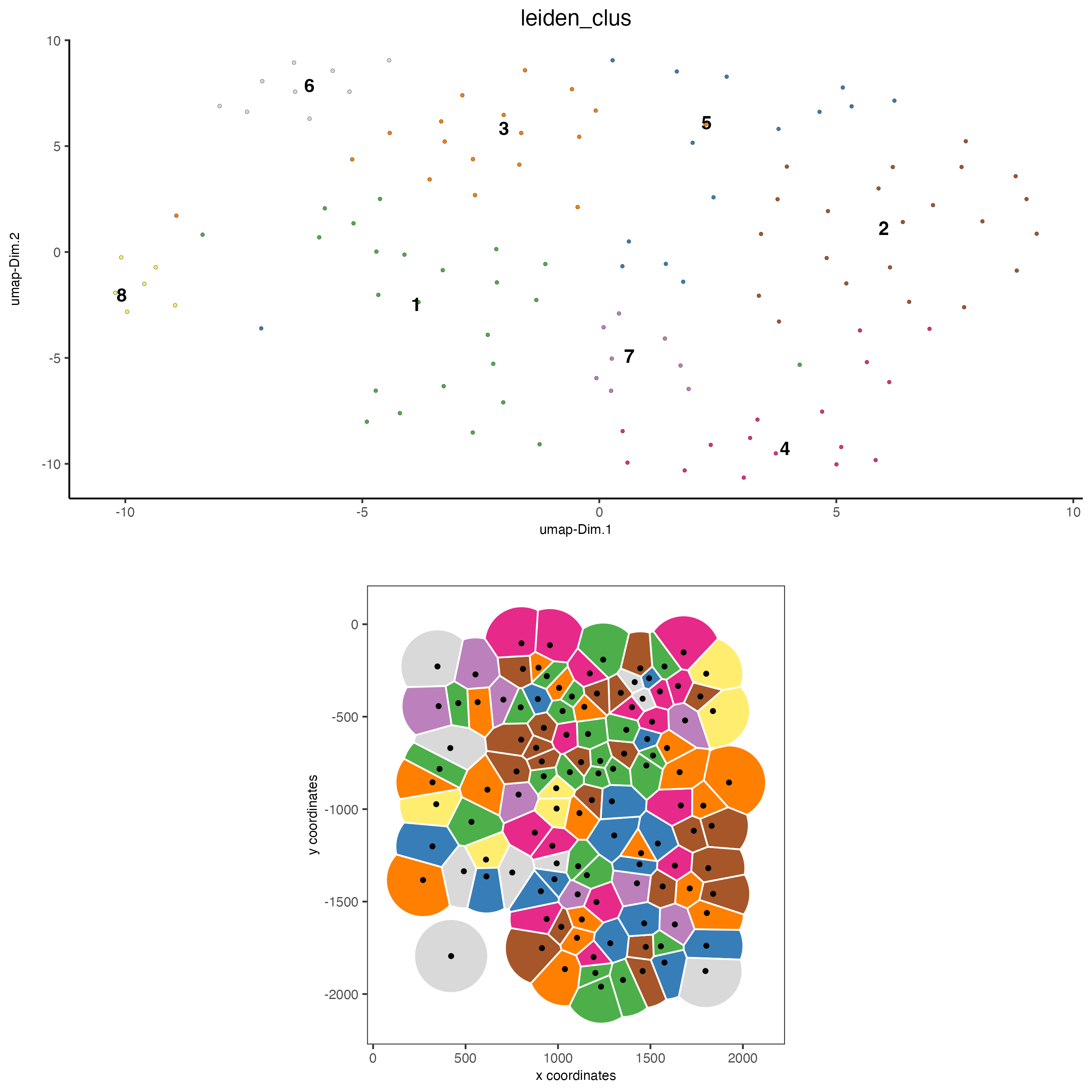
# heatmap and dendrogram
showClusterHeatmap(gobject = seqfish_mini,
                   cluster_column = "leiden_clus")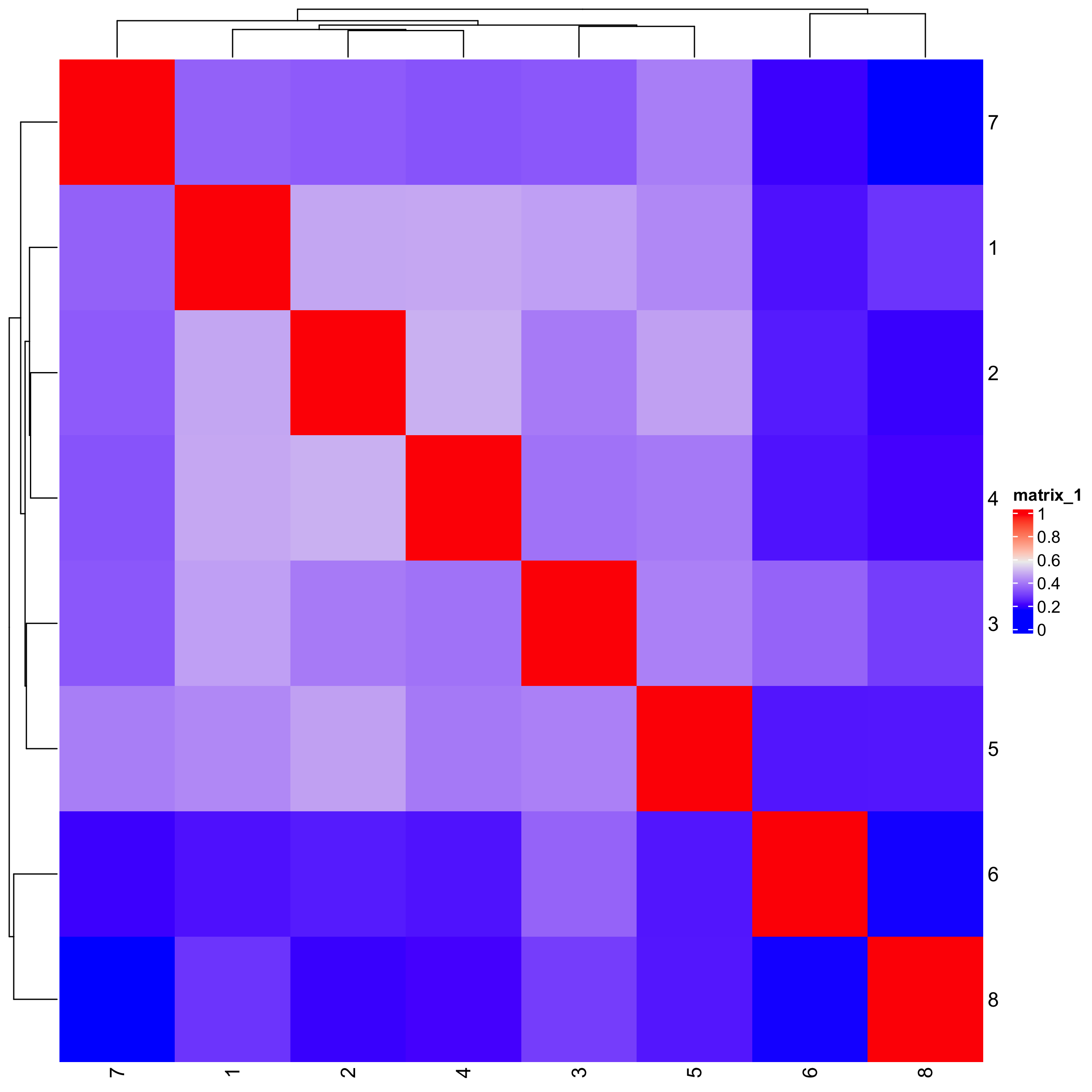
The following step requires the installation of {ggdendro}.
# install.packages("ggdendro")
library(ggdendro)

showClusterDendrogram(seqfish_mini,
                      h = 0.5,
                      rotate = TRUE,
                      cluster_column = "leiden_clus")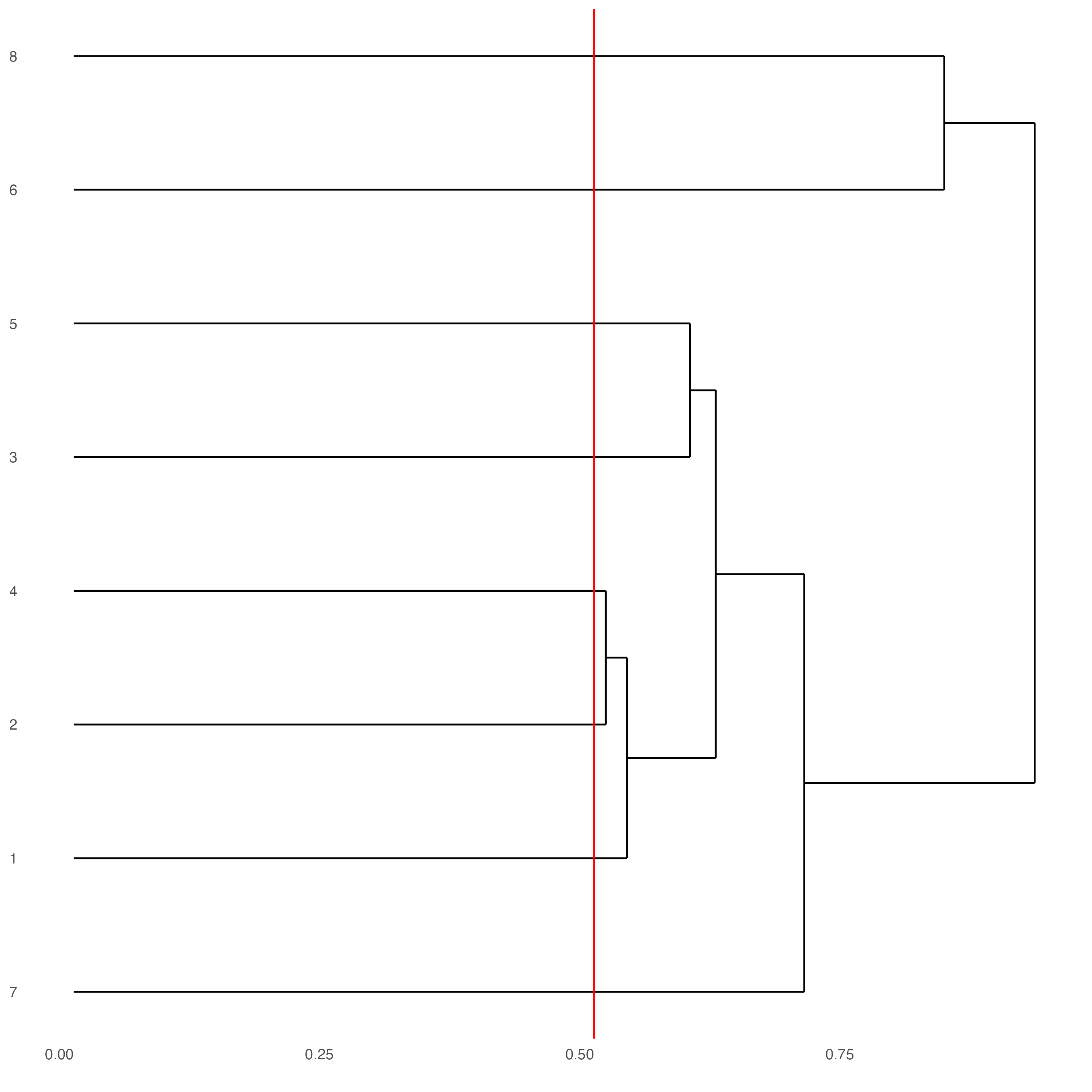
6 Differential expression
markers_gini <- findMarkers_one_vs_all(gobject = seqfish_mini,
                                       method = "gini",
                                       expression_values = "normalized",
                                       cluster_column = "leiden_clus",
                                       min_feats = 20,
                                       min_expr_gini_score = 0.5,
                                       min_det_gini_score = 0.5)

# get top 2 genes per cluster and visualize with violin plot
topgenes_gini = markers_gini[, head(.SD, 2), by = "cluster"]

violinPlot(seqfish_mini,
           feats = topgenes_gini$feats[1:4],
           cluster_column = "leiden_clus")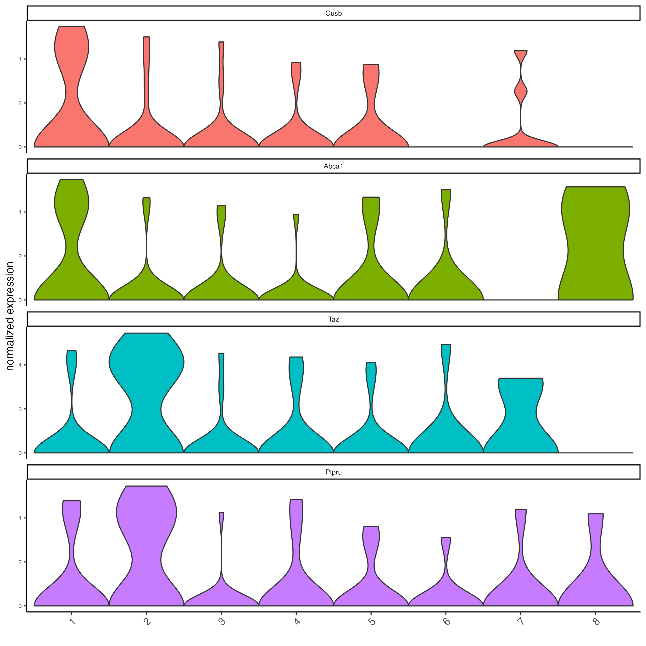
# get top 6 genes per cluster and visualize with heatmap
topgenes_gini <- markers_gini[, head(.SD, 6), by = "cluster"]

plotMetaDataHeatmap(seqfish_mini,
                    selected_feats = topgenes_gini$feats,
                    metadata_cols = "leiden_clus")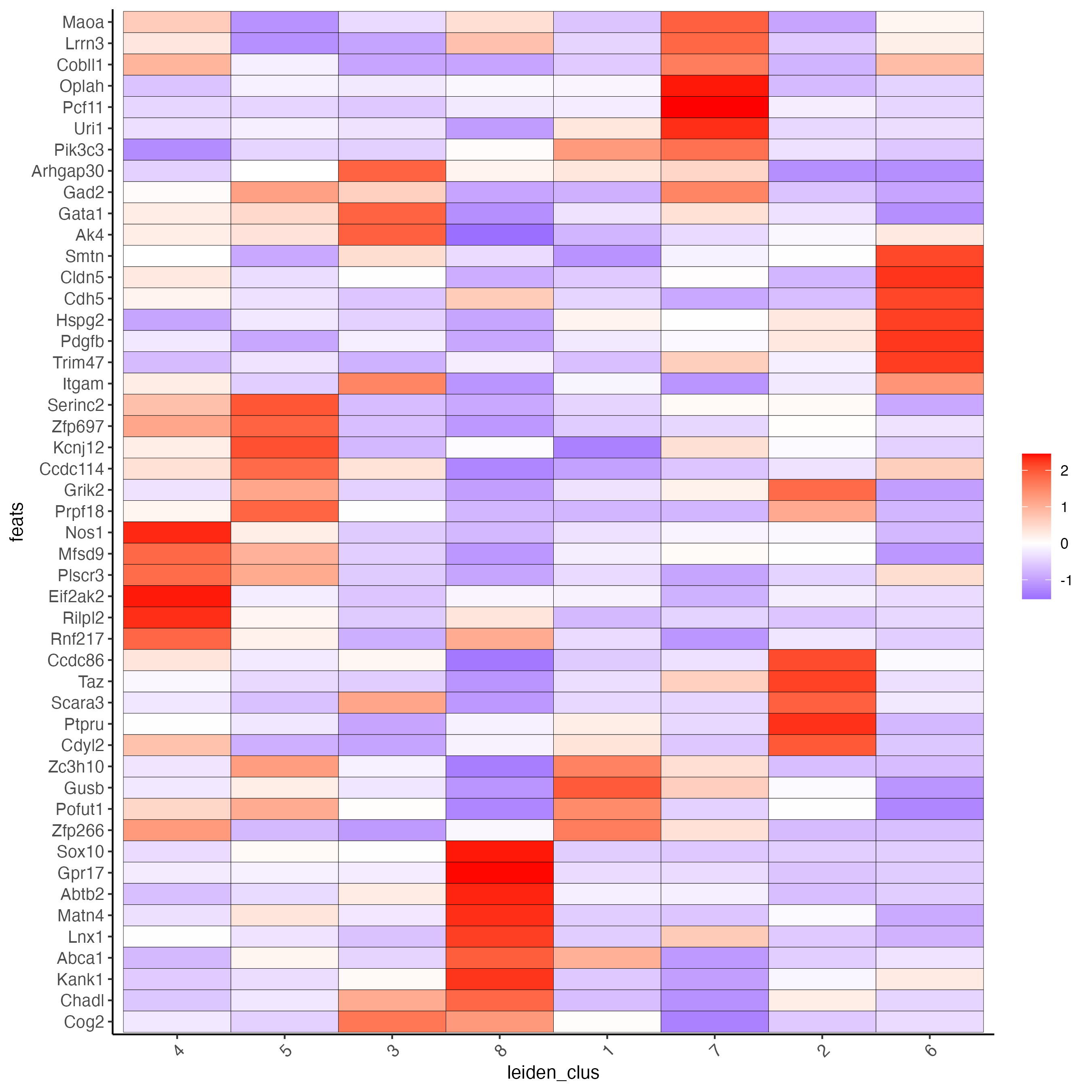
7 Cell type annotation
clusters_cell_types <- c("cell A", "cell B", "cell C", "cell D",
                        "cell E", "cell F", "cell G", "cell H")

names(clusters_cell_types) <- 1:8

seqfish_mini <- annotateGiotto(gobject = seqfish_mini,
                               annotation_vector = clusters_cell_types,
                               cluster_column = "leiden_clus",
                               name = "cell_types")

# check new cell metadata
pDataDT(seqfish_mini)

# visualize annotations
spatDimPlot(gobject = seqfish_mini,
            cell_color = "cell_types",
            spat_point_size = 3,
            dim_point_size = 3)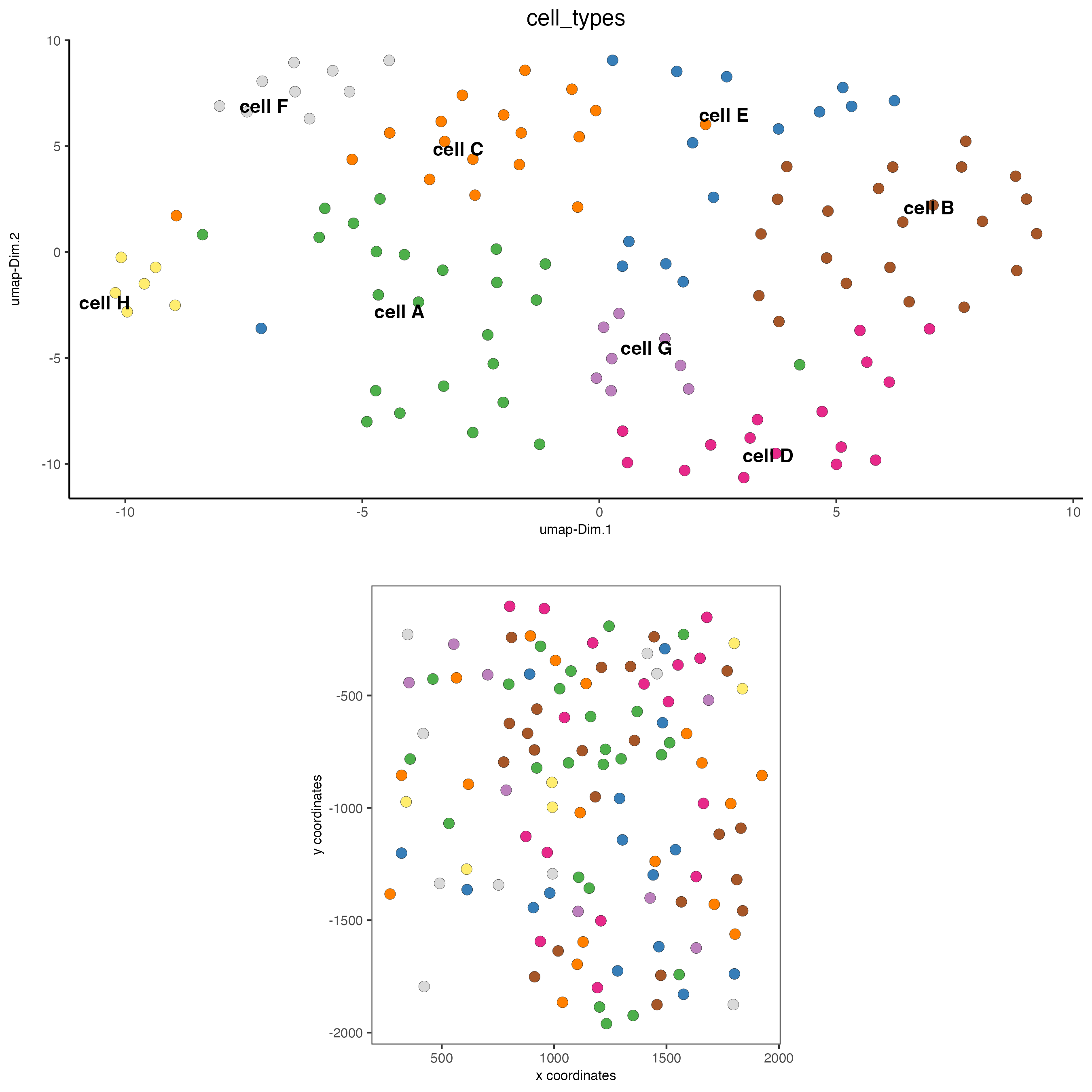
# heatmap
topgenes_heatmap <- markers_gini[, head(.SD, 4), by = "cluster"]

plotHeatmap(gobject = seqfish_mini,
            feats = topgenes_heatmap$feats,
            feat_order = "custom",
            feat_custom_order = unique(topgenes_heatmap$feats),
            cluster_column = "cell_types",
            legend_nrows = 1)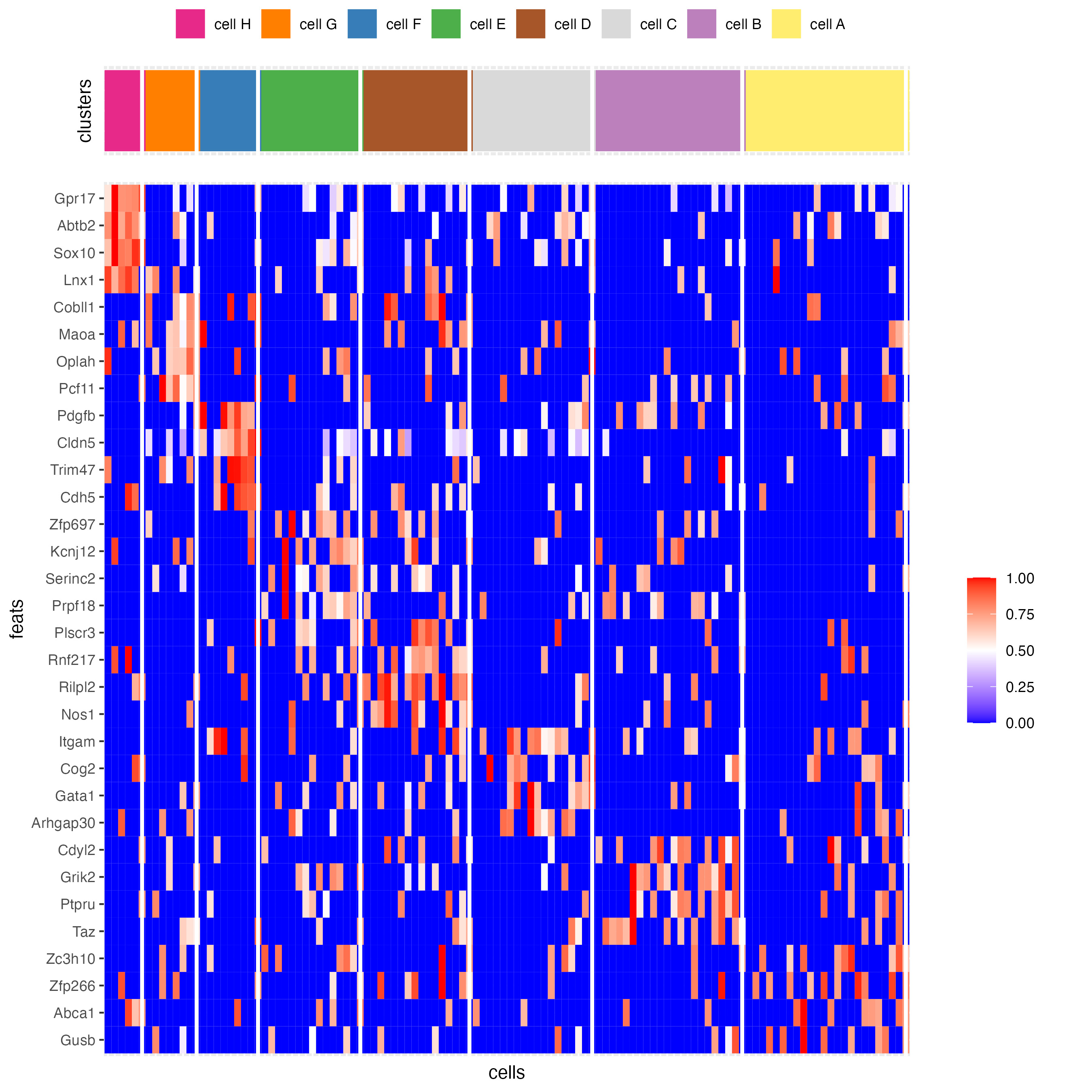
8 Spatial grid
- Create a grid based on defined step sizes in the x,y(,z) axes.
seqfish_mini <- createSpatialGrid(gobject = seqfish_mini,
                                  sdimx_stepsize = 300,
                                  sdimy_stepsize = 300,
                                  minimum_padding = 50)

showGiottoSpatGrids(seqfish_mini)

# visualize grid
spatPlot(gobject = seqfish_mini,
         show_grid = TRUE,
         point_size = 1.5)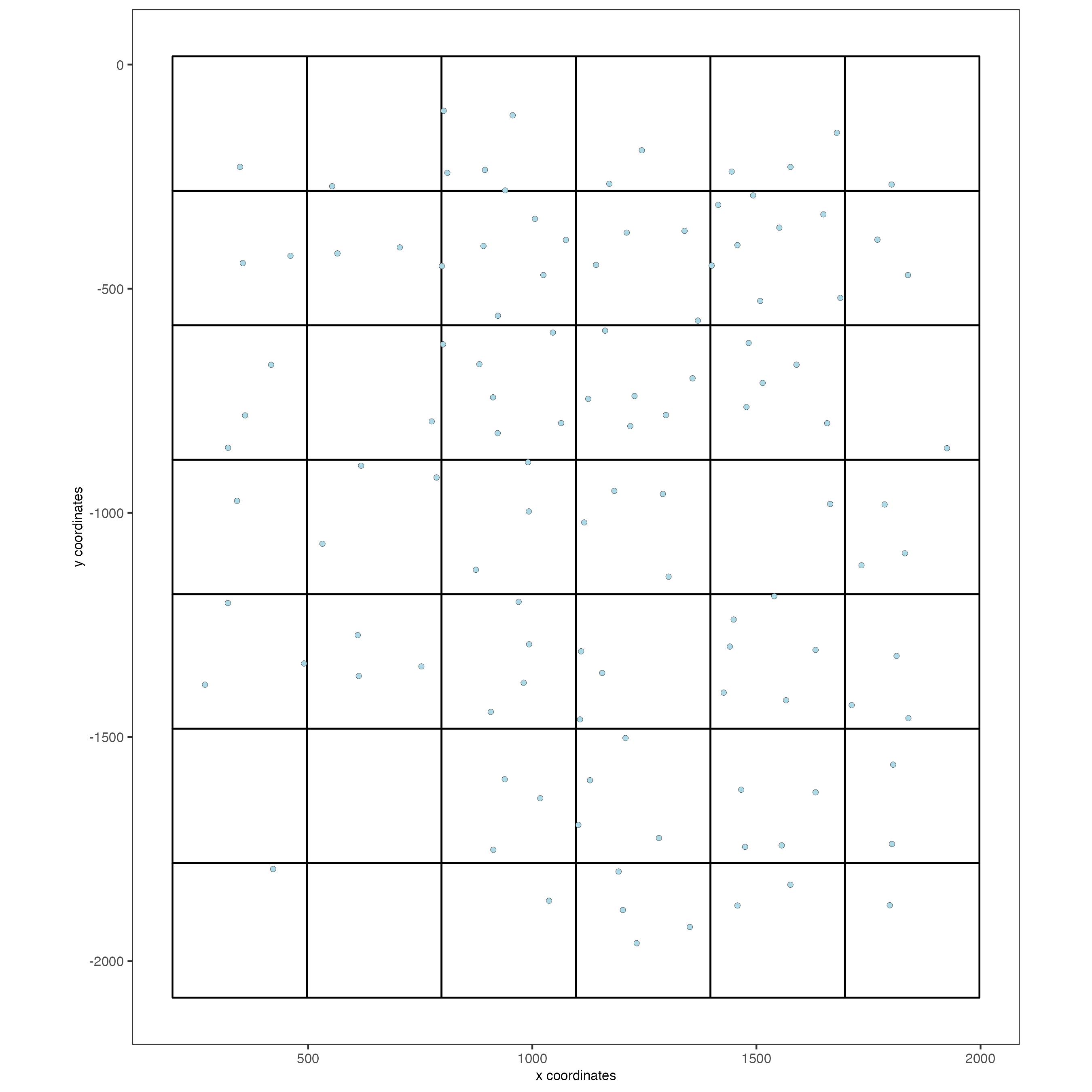
9 Spatial network
- Visualize information about the default Delaunay network
- Create a spatial Delaunay network (default)
- Create a spatial kNN network
plotStatDelaunayNetwork(gobject = seqfish_mini,
                        maximum_distance = 400)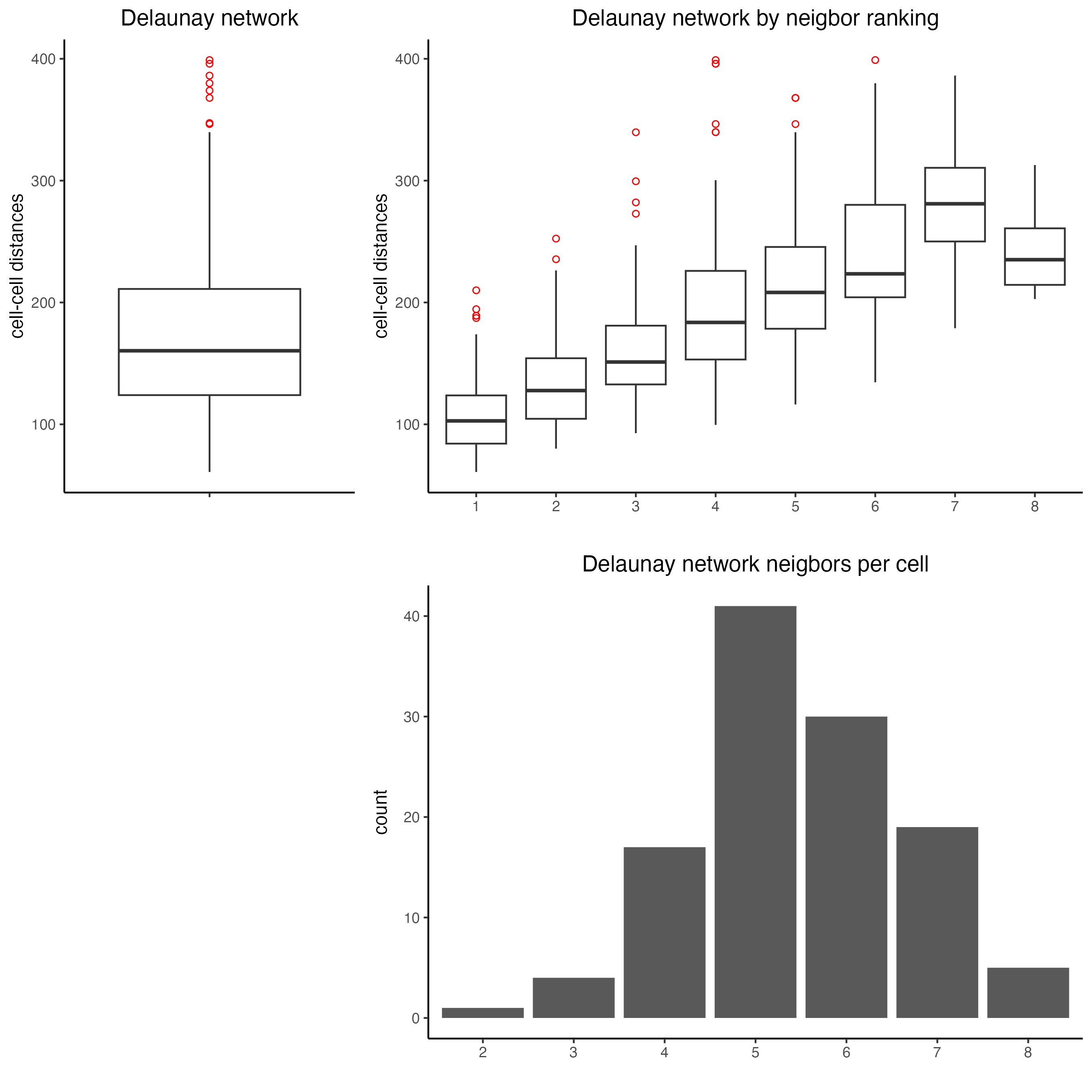
seqfish_mini <- createSpatialNetwork(gobject = seqfish_mini,
                                     minimum_k = 2,
                                     maximum_distance_delaunay = 400)

seqfish_mini <- createSpatialNetwork(gobject = seqfish_mini,
                                     minimum_k = 2,
                                     method = "kNN",
                                     k = 10)

showGiottoSpatNetworks(seqfish_mini)

# visualize the two different spatial networks
spatPlot(gobject = seqfish_mini,
         show_network = TRUE,
         network_color = "blue",
         spatial_network_name = "Delaunay_network",
         point_size = 2.5,
         cell_color = "leiden_clus")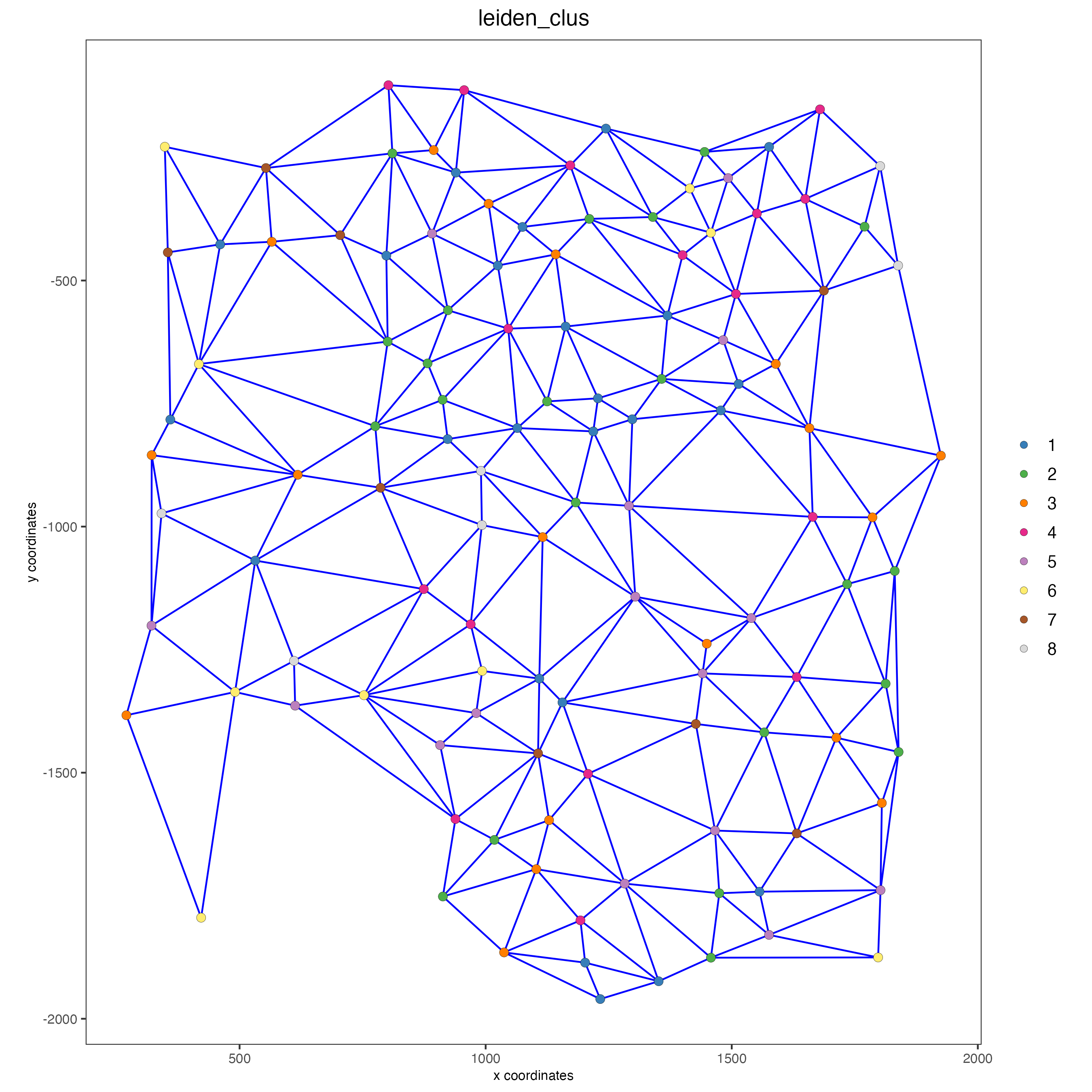
spatPlot(gobject = seqfish_mini,
         show_network = TRUE,
         network_color = "blue",
         spatial_network_name = "kNN_network",
         point_size = 2.5,
         cell_color = "leiden_clus")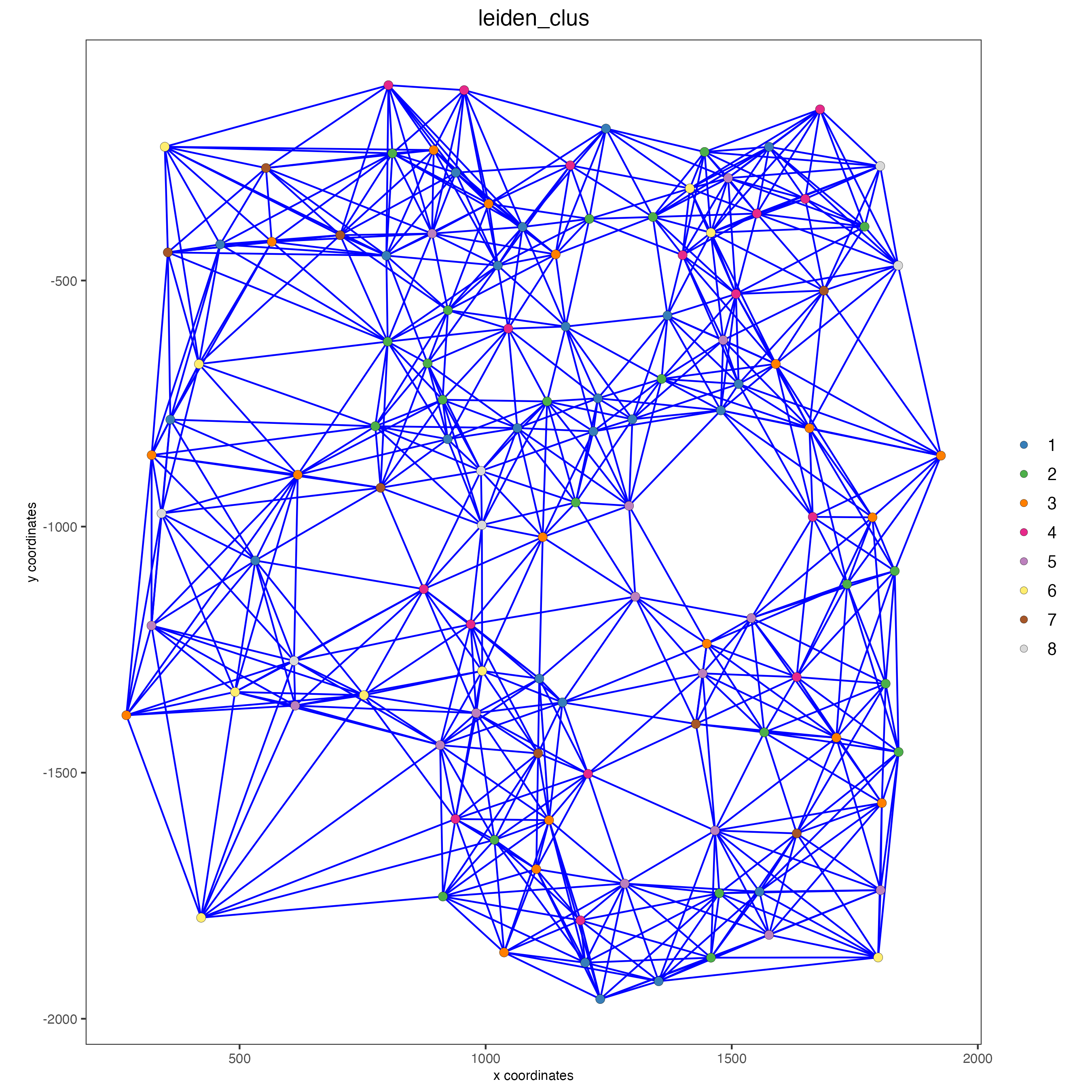
10 Spatial genes
Identify spatial genes with 3 different methods:
- binSpect with k-means binarization (default)
- binSpect with rank binarization
- silhouetteRank
Visualize top 4 genes per method.
km_spatialfeats <- binSpect(seqfish_mini)

spatFeatPlot2D(seqfish_mini,
               expression_values = "scaled",
               feats = km_spatialfeats[1:4]$feats,
               point_shape = "border",
               point_border_stroke = 0.1,
               show_network = FALSE,
               network_color = "lightgrey",
               point_size = 2.5,
               cow_n_col = 2)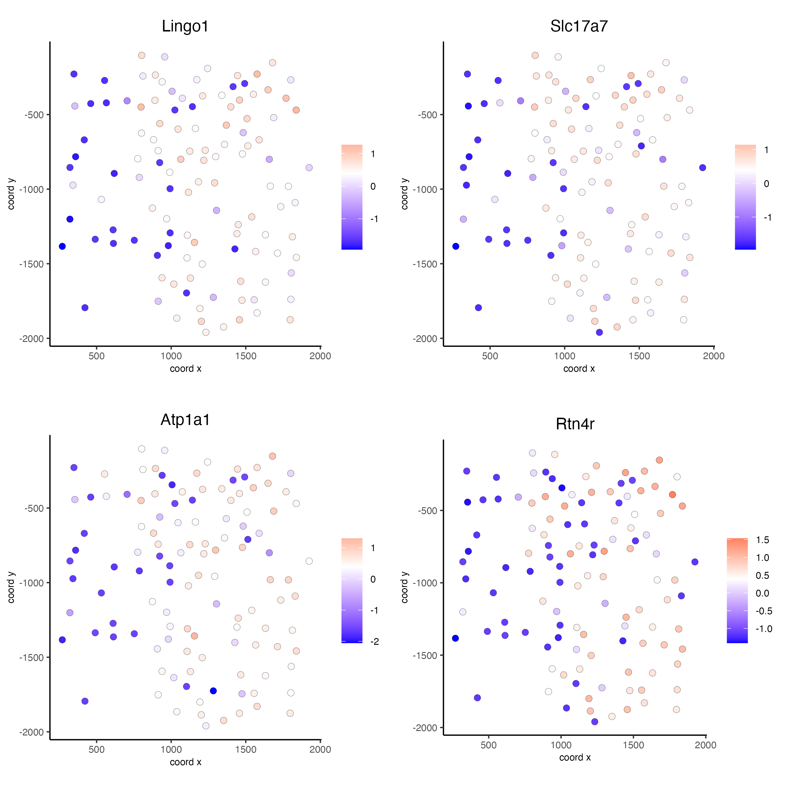
rank_spatialgenes <- binSpect(seqfish_mini,
                              bin_method = "rank")

spatFeatPlot2D(seqfish_mini,
               expression_values = "scaled",
               feats = rank_spatialgenes[1:4]$feats,
               point_shape = "border",
               point_border_stroke = 0.1,
               show_network = FALSE,
               network_color = "lightgrey",
               point_size = 2.5,
               cow_n_col = 2)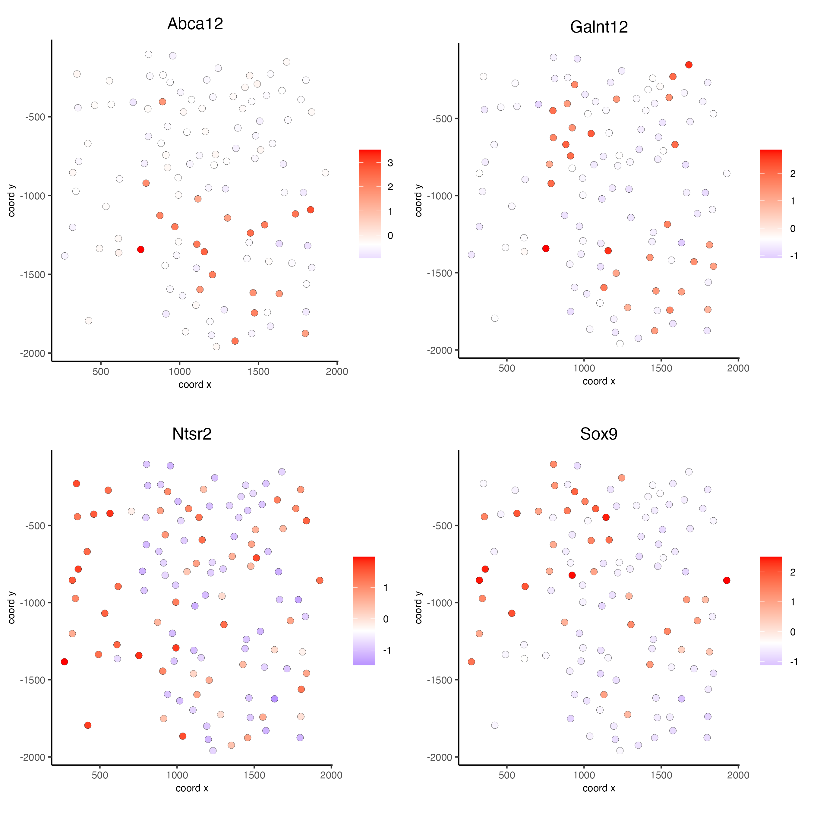
silh_spatialgenes <- silhouetteRank(gobject = seqfish_mini) # TODO: suppress print output

spatFeatPlot2D(seqfish_mini,
               expression_values = "scaled",
               feats = silh_spatialgenes[1:4]$genes,
               point_shape = "border",
               point_border_stroke = 0.1,
               show_network = FALSE,
               network_color = "lightgrey",
               point_size = 2.5,
               cow_n_col = 2)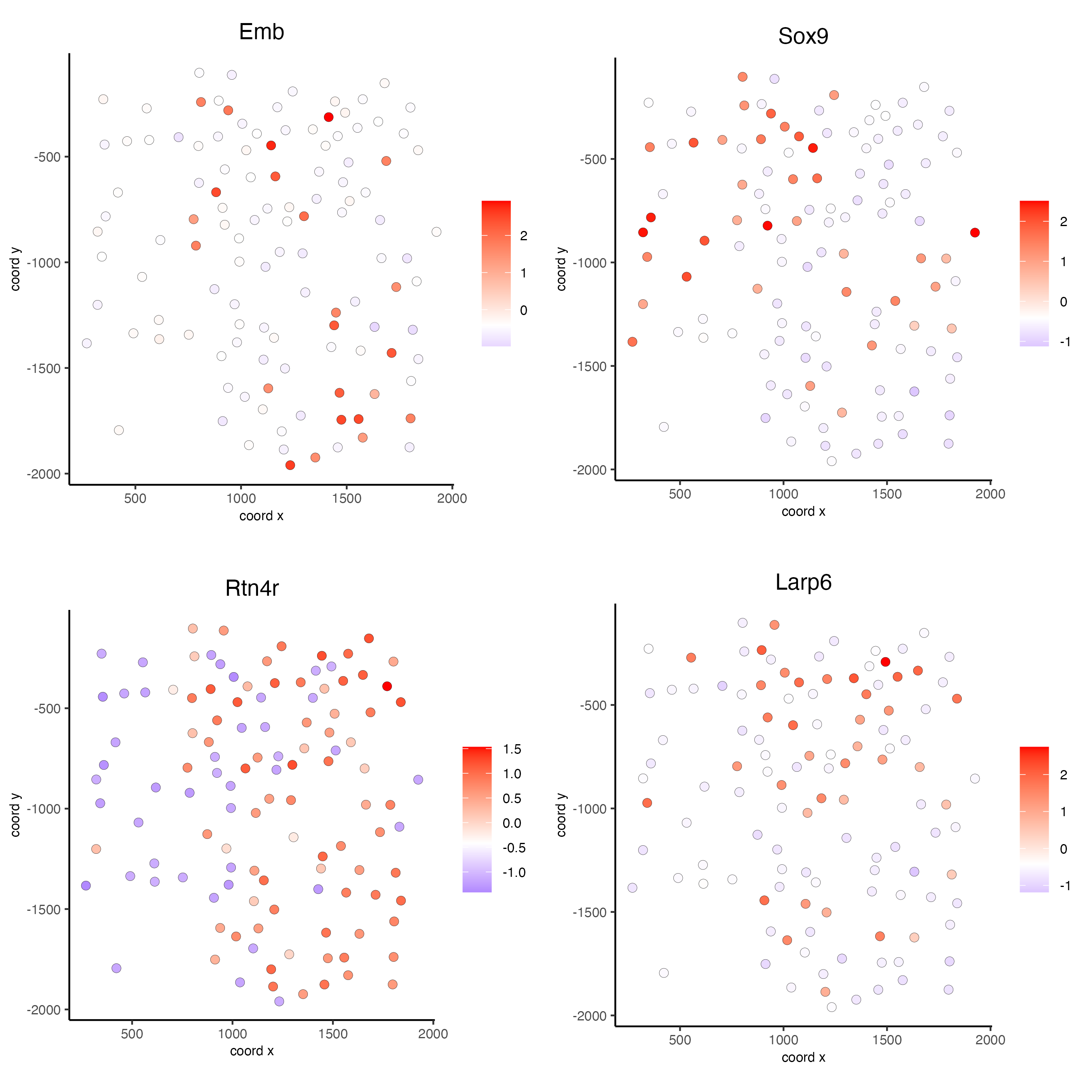
11 Spatial co-expression patterns
Identify robust spatial co-expression patterns using the spatial network or grid and a subset of individual spatial genes.
- Calculate spatial correlation scores
- Cluster correlation scores
# 1. calculate spatial correlation scores
ext_spatial_genes <- km_spatialfeats[1:500]$feats

spat_cor_netw_DT <- detectSpatialCorFeats(seqfish_mini,
                                          method = "network",
                                          spatial_network_name = "Delaunay_network",
                                          subset_feats = ext_spatial_genes)

# 2. cluster correlation scores
spat_cor_netw_DT <- clusterSpatialCorFeats(spat_cor_netw_DT,
                                           name = "spat_netw_clus",
                                           k = 8)

heatmSpatialCorFeats(seqfish_mini,
                     spatCorObject = spat_cor_netw_DT,
                     use_clus_name = "spat_netw_clus")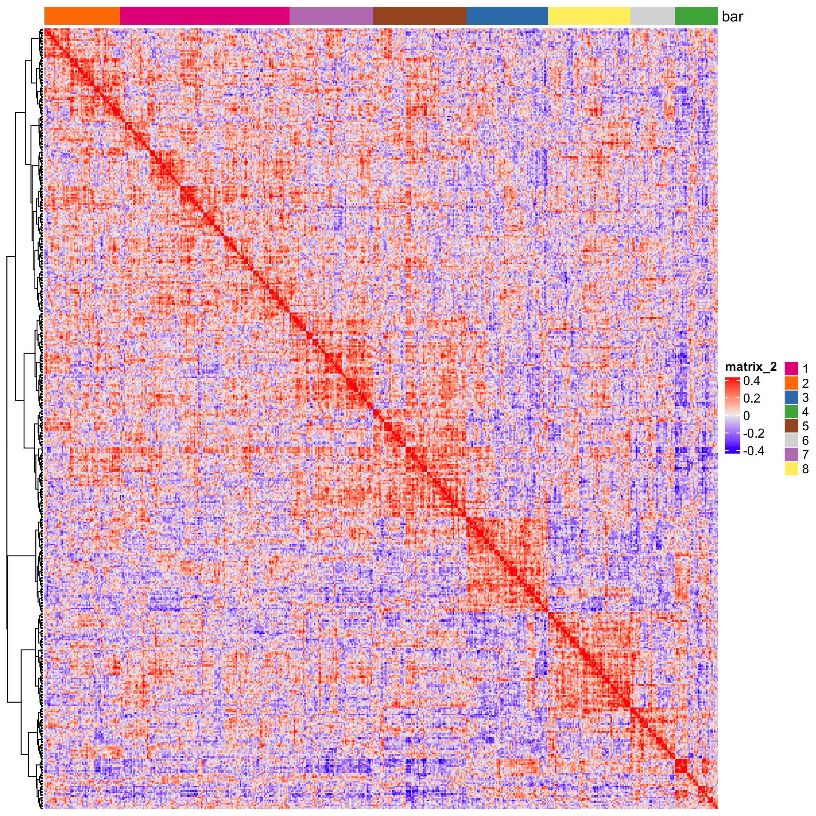
netw_ranks <- rankSpatialCorGroups(seqfish_mini,
                                   spatCorObject = spat_cor_netw_DT,
                                   use_clus_name = "spat_netw_clus")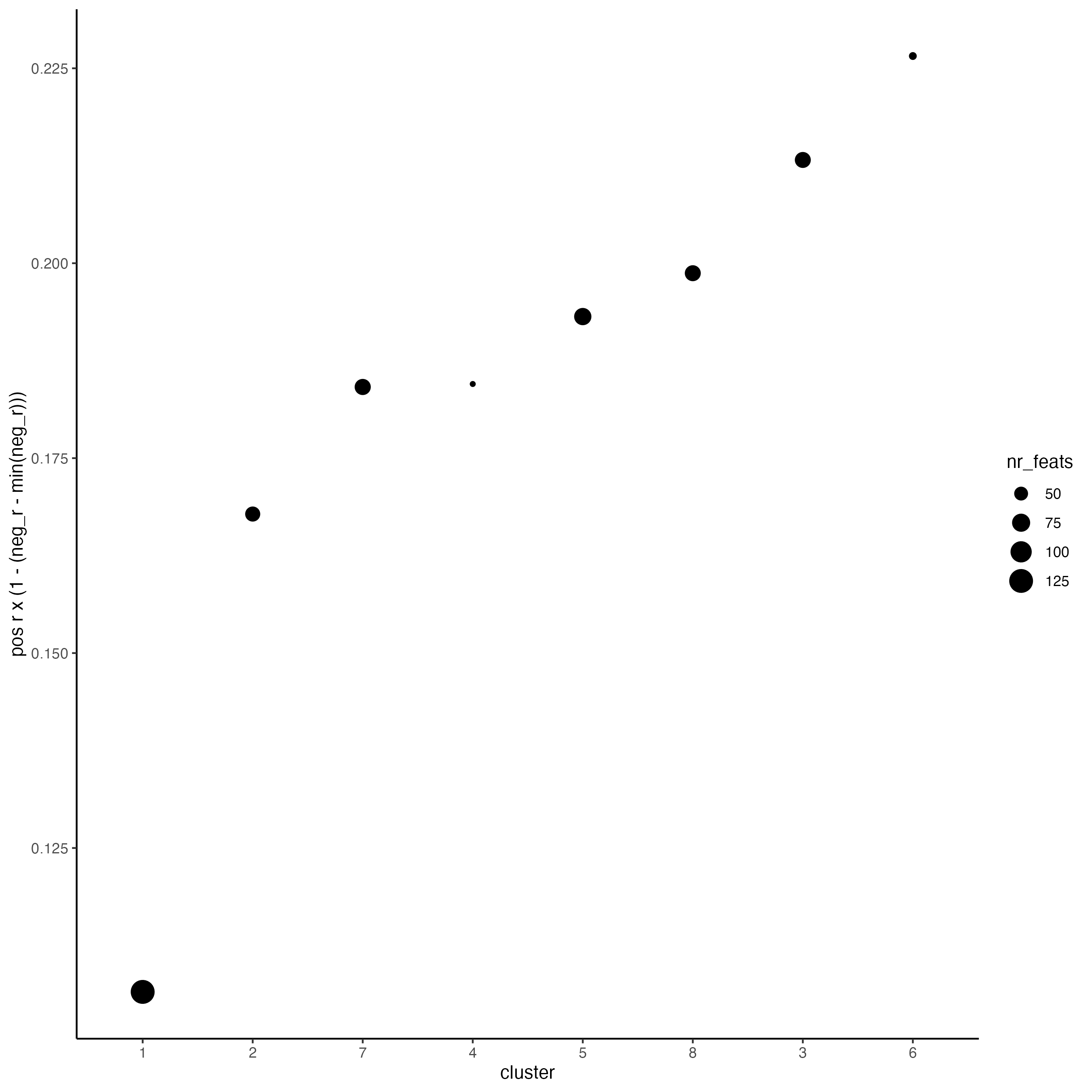
top_netw_spat_cluster <- showSpatialCorFeats(spat_cor_netw_DT,
                                             use_clus_name = "spat_netw_clus",
                                             selected_clusters = 6,
                                             show_top_feats = 1)

cluster_genes_DT <- showSpatialCorFeats(spat_cor_netw_DT,
                                        use_clus_name = "spat_netw_clus",
                                        show_top_feats = 1)

cluster_genes <- cluster_genes_DT$clus
names(cluster_genes) <- cluster_genes_DT$feat_ID

seqfish_mini <- createMetafeats(seqfish_mini,
                                feat_clusters = cluster_genes,
                                name = "cluster_metagene")

spatCellPlot(seqfish_mini,
             spat_enr_names = "cluster_metagene",
             cell_annotation_values = netw_ranks$clusters,
             point_size = 1.5,
             cow_n_col = 3)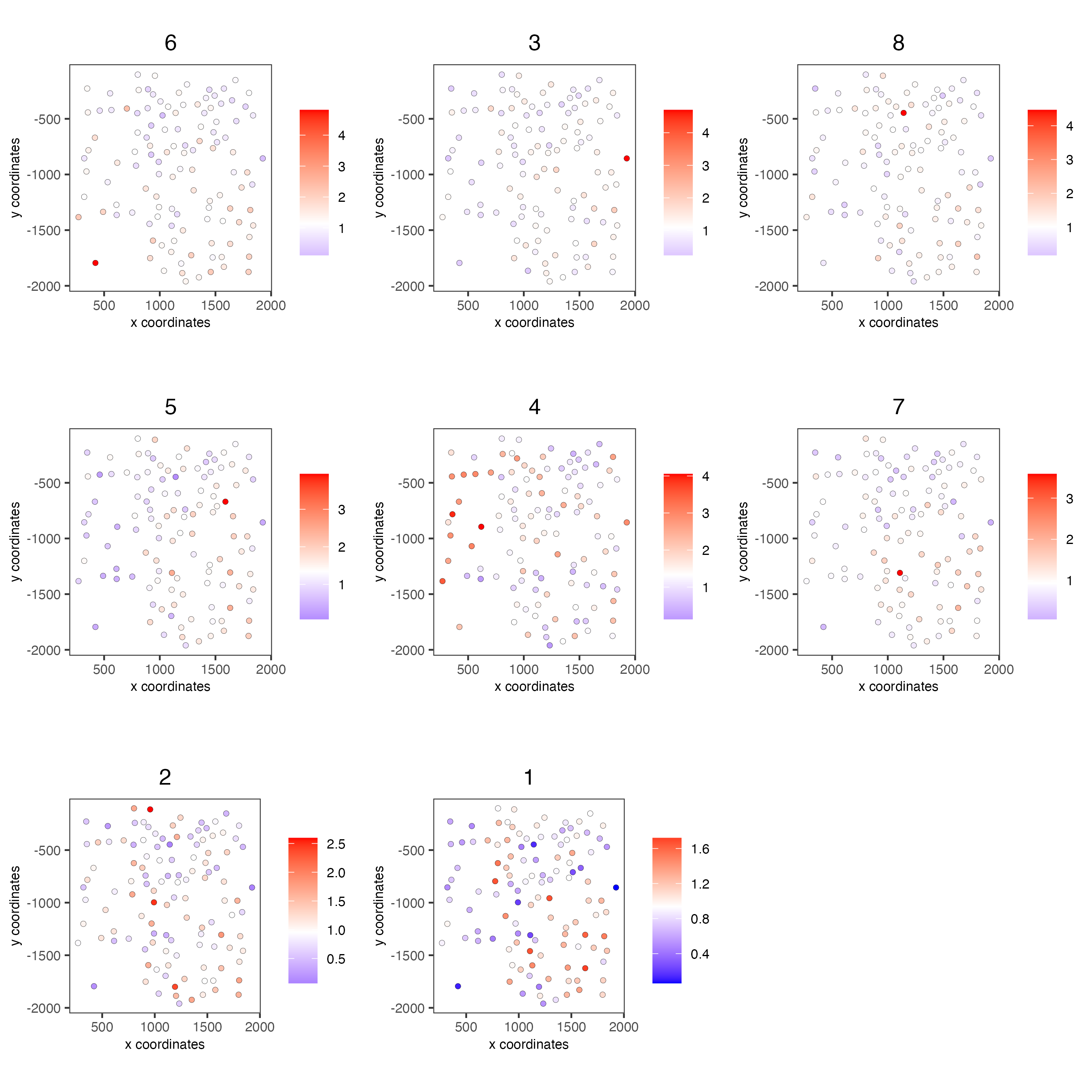
12 Spatial HMRF domains
The following HMRF function requires {smfishHmrf} .
# remotes::install_bitbucket(repo = "qzhudfci/smfishhmrf-r", ref="master")
library(smfishHmrf)

hmrf_folder <- paste0(results_folder, "/11_HMRF/")

if(!file.exists(hmrf_folder)) dir.create(hmrf_folder, recursive = TRUE)

# perform hmrf
my_spatial_genes <- km_spatialfeats[1:100]$feats

HMRF_spatial_genes <- doHMRF(gobject = seqfish_mini,
                            expression_values = "scaled",
                            spatial_genes = my_spatial_genes,
                            spatial_network_name = "Delaunay_network",
                            k = 9,
                            betas = c(28,2,2),
                            output_folder = paste0(hmrf_folder, "/", "Spatial_genes/SG_top100_k9_scaled"))

# check and select hmrf
for(i in seq(28, 30, by = 2)) {
  viewHMRFresults2D(gobject = seqfish_mini,
                    HMRFoutput = HMRF_spatial_genes,
                    k = 9,
                    betas_to_view = i,
                    point_size = 2)
}

seqfish_mini <- addHMRF(gobject = seqfish_mini,
                        HMRFoutput = HMRF_spatial_genes,
                        k = 9,
                        betas_to_add = 28,
                        hmrf_name = "HMRF")

# visualize selected hmrf result
giotto_colors <- getDistinctColors(9)
names(giotto_colors) <- 1:9

spatPlot(gobject = seqfish_mini,
         cell_color = "HMRF_k9_b.28",
         point_size = 3,
         coord_fix_ratio = 1,
         cell_color_code = giotto_colors)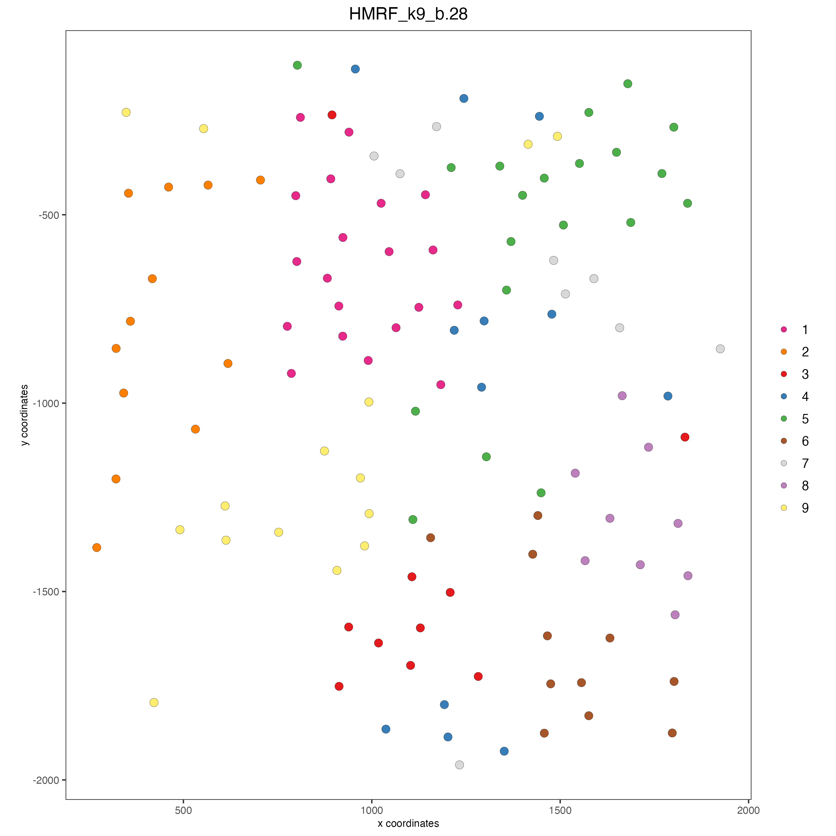
13 Cell neighborhood: cell-type/cell-type interactions
set.seed(seed = 2841)

cell_proximities <- cellProximityEnrichment(gobject = seqfish_mini,
                                            cluster_column = "cell_types",
                                            spatial_network_name = "Delaunay_network",
                                            adjust_method = "fdr",
                                            number_of_simulations = 1000)

# barplot
cellProximityBarplot(gobject = seqfish_mini,
                     CPscore = cell_proximities,
                     min_orig_ints = 5,
                     min_sim_ints = 5,
                     p_val = 0.5)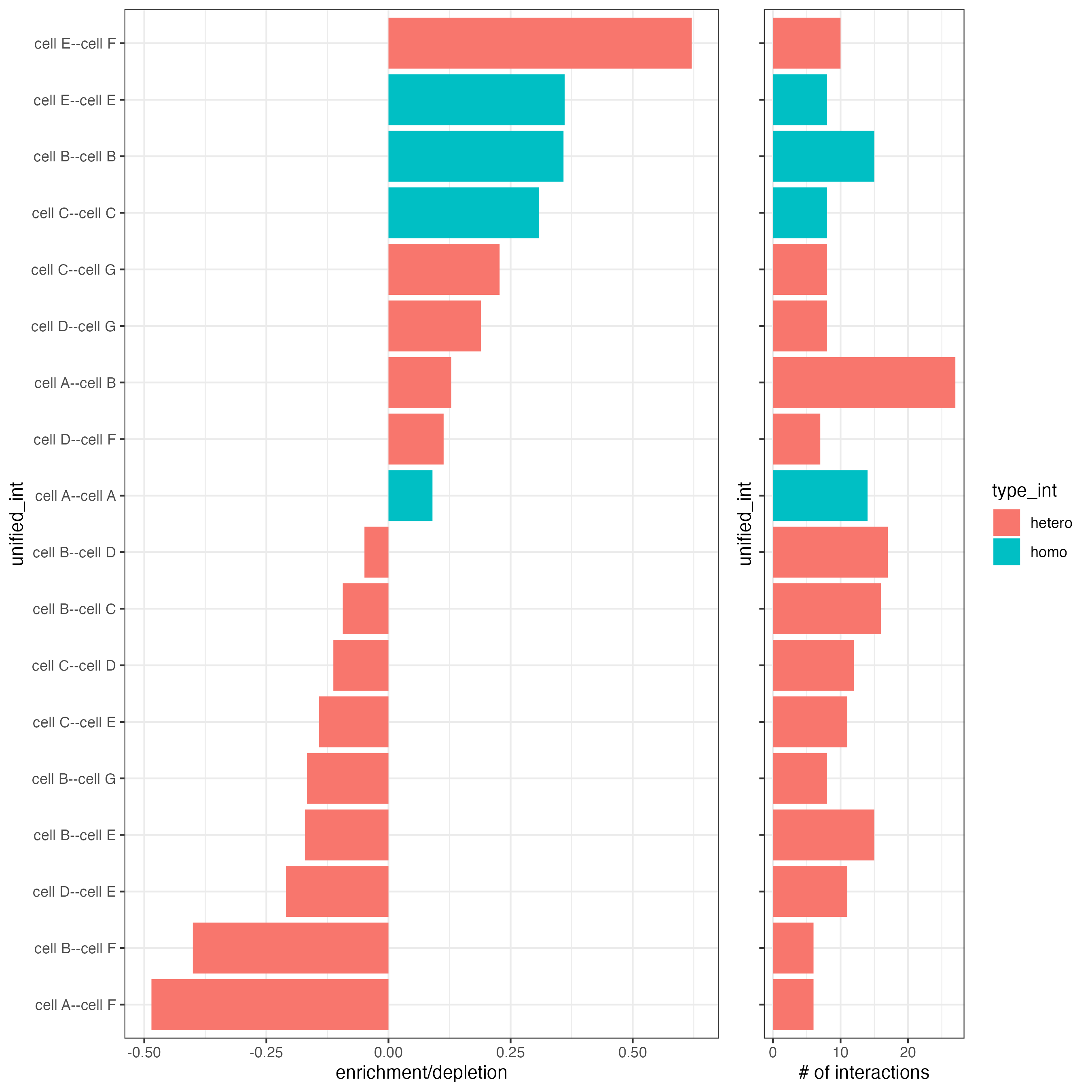
## heatmap
cellProximityHeatmap(gobject = seqfish_mini,
                     CPscore = cell_proximities,
                     order_cell_types = TRUE,
                     scale = TRUE,
                     color_breaks = c(-1.5, 0, 1.5),
                     color_names = c("blue", "white", "red"))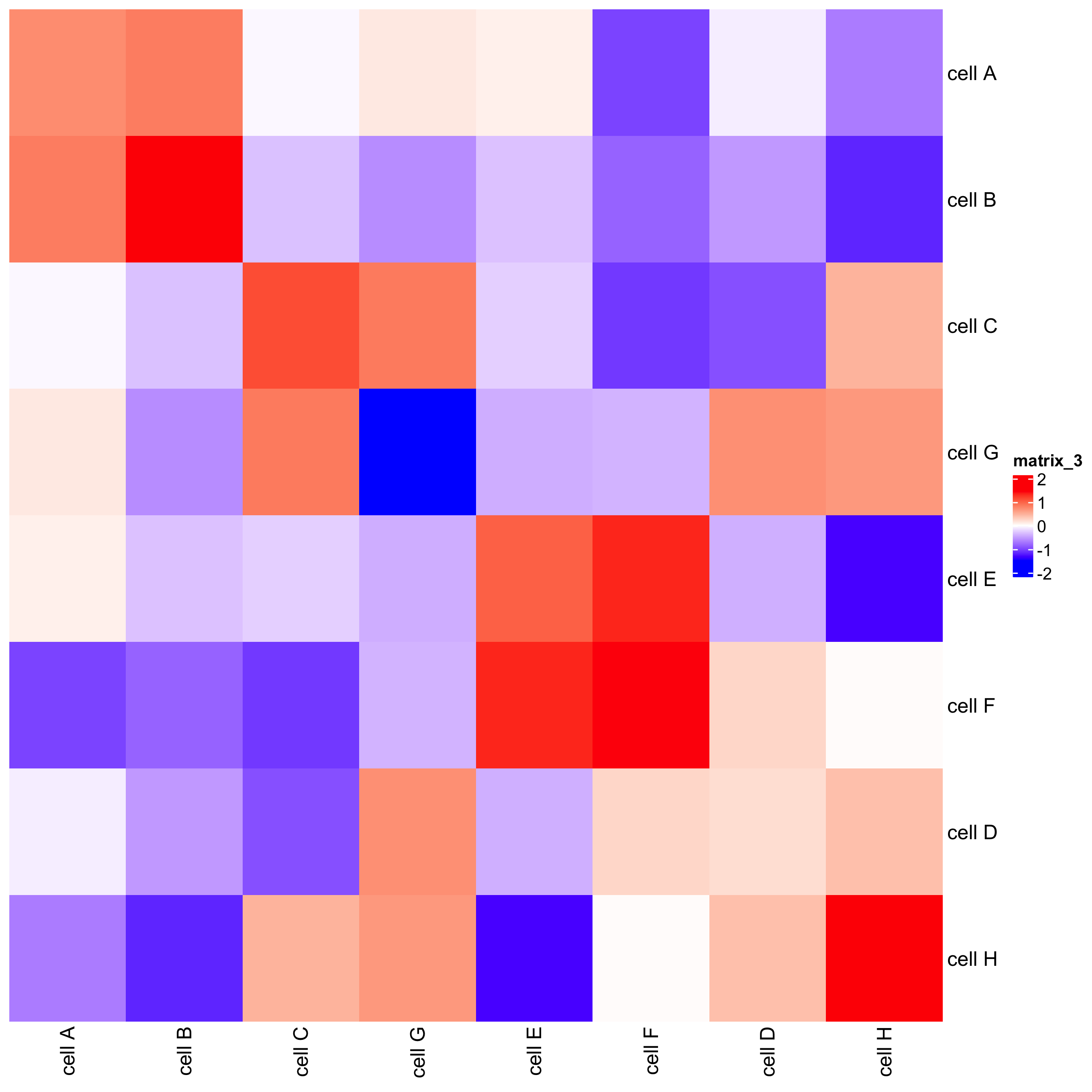
# network
cellProximityNetwork(gobject = seqfish_mini,
                     CPscore = cell_proximities,
                     remove_self_edges = TRUE,
                     only_show_enrichment_edges = TRUE)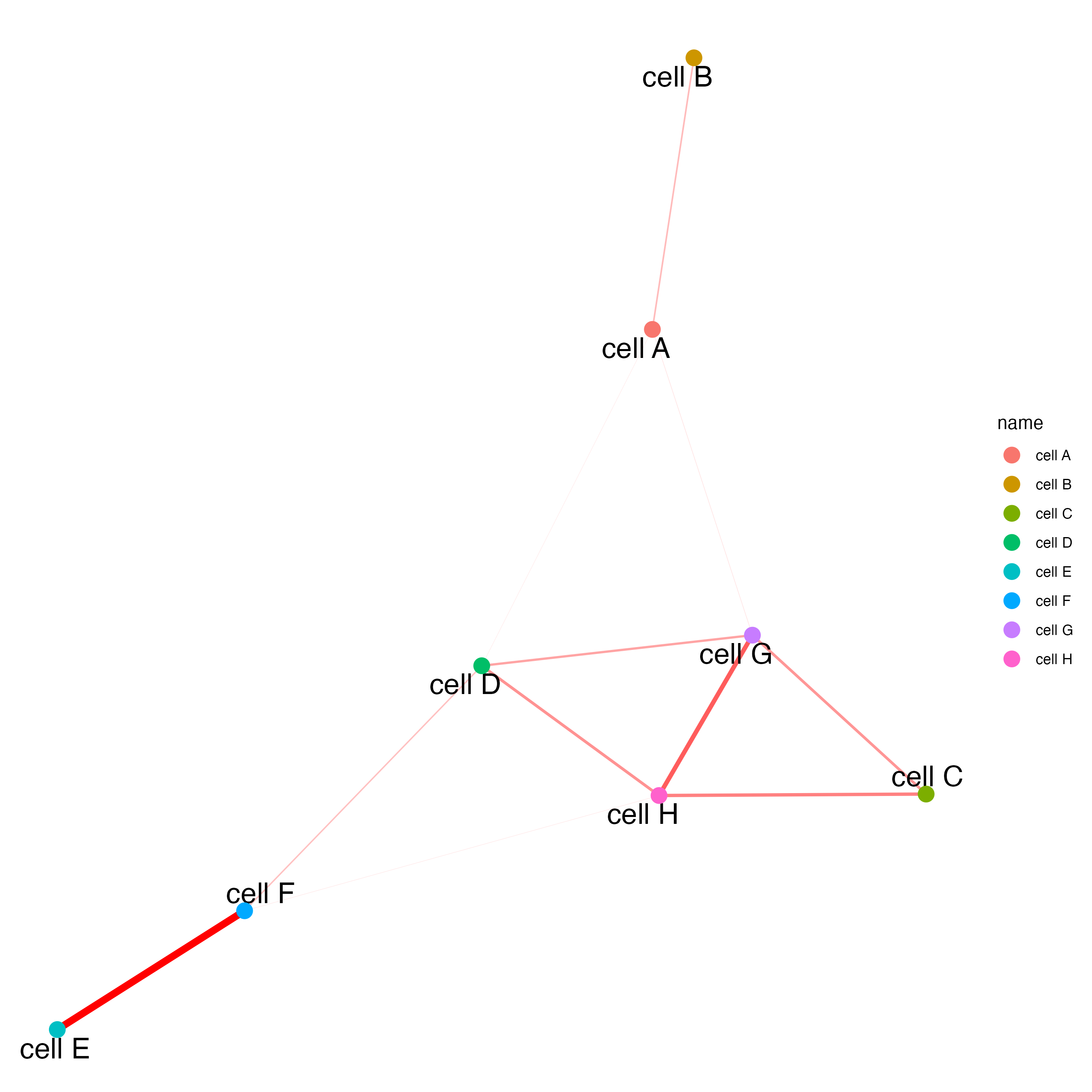
# network with self-edges
cellProximityNetwork(gobject = seqfish_mini,
                     CPscore = cell_proximities,
                     remove_self_edges = FALSE,
                     self_loop_strength = 0.3,
                     only_show_enrichment_edges = FALSE,
                     rescale_edge_weights = TRUE,
                     node_size = 8,
                     edge_weight_range_depletion = c(1, 2),
                     edge_weight_range_enrichment = c(2,5))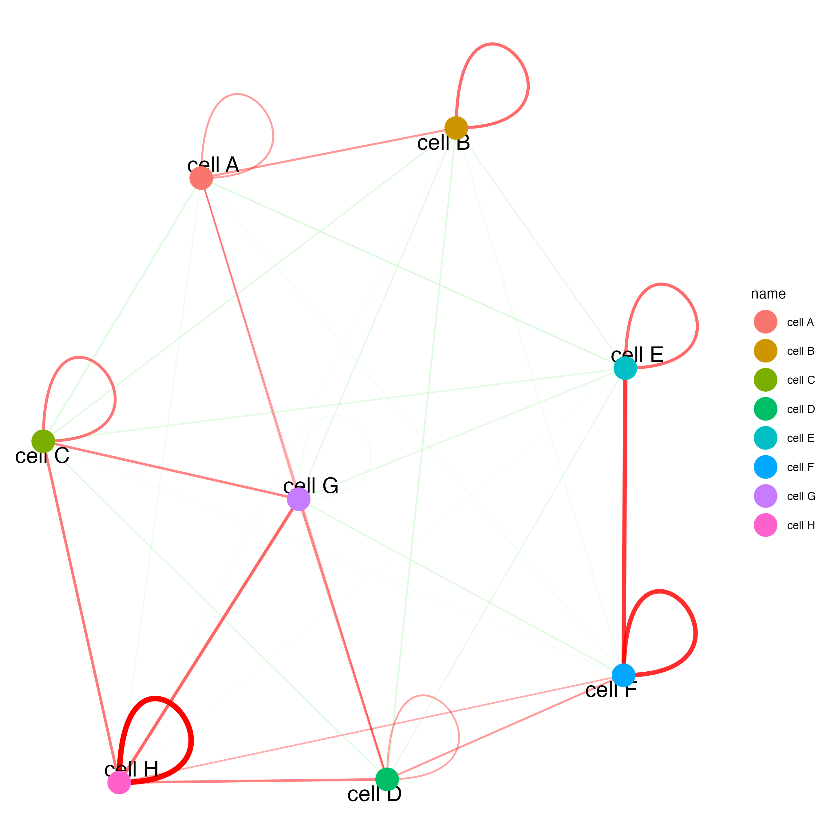
13.1 Visualization of specific cell types
# Option 1
spec_interaction <- "cell D--cell F"

cellProximitySpatPlot2D(gobject = seqfish_mini,
                        interaction_name = spec_interaction,
                        show_network = TRUE,
                        cluster_column = "cell_types",
                        cell_color = "cell_types",
                        cell_color_code = c("cell D" = "lightblue", "cell F" = "red"),
                        point_size_select = 4,
                        point_size_other = 2)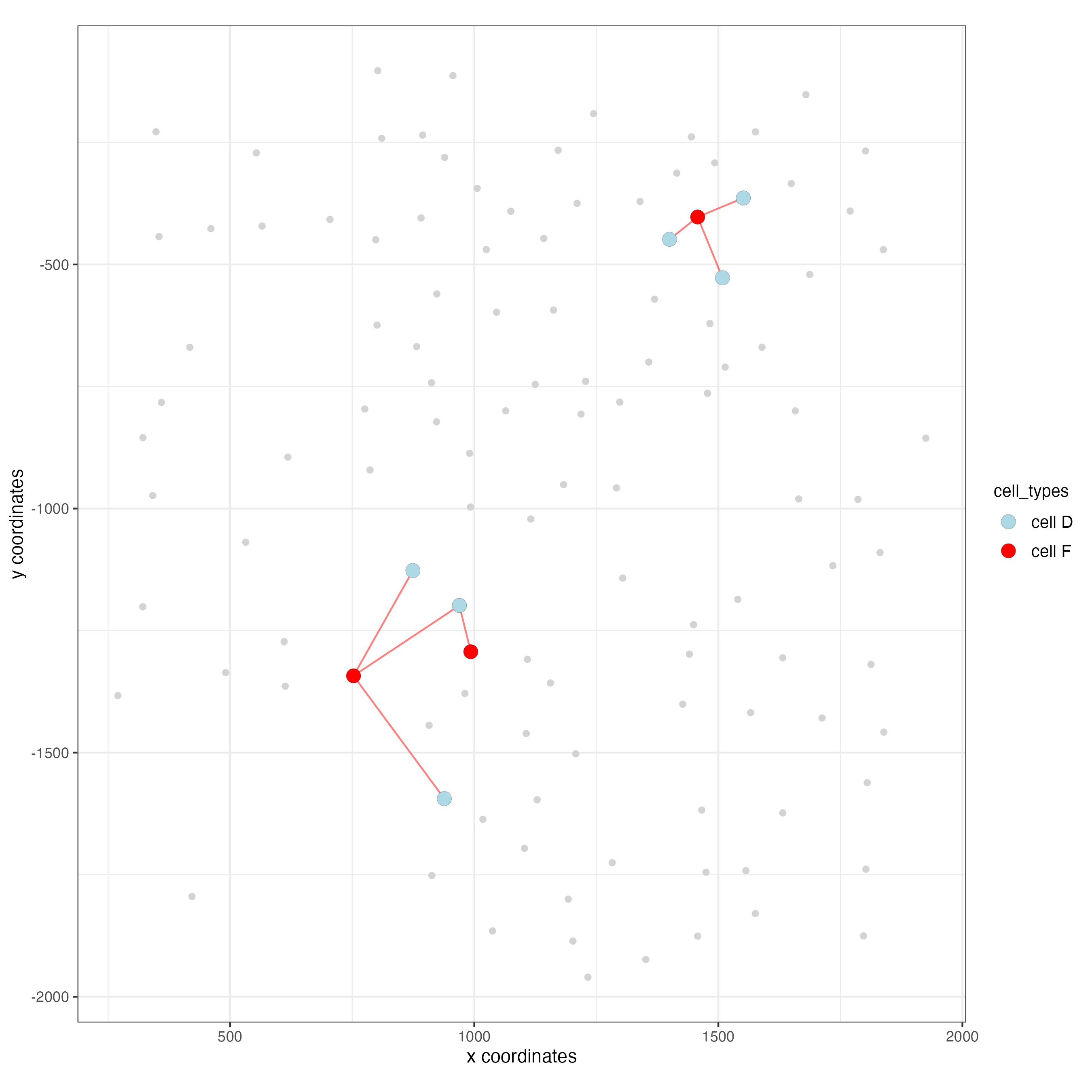
# Option 2: create additional metadata
seqfish_mini <- addCellIntMetadata(seqfish_mini,
                                   spat_unit = "cell",
                                   spatial_network = "Delaunay_network",
                                   cluster_column = "cell_types",
                                   cell_interaction = spec_interaction,
                                   name = "D_F_interactions")

spatPlot(seqfish_mini,
         cell_color = "D_F_interactions",
         legend_symbol_size = 3,
         select_cell_groups =  c("other_cell D", "other_cell F", "select_cell D", "select_cell F"))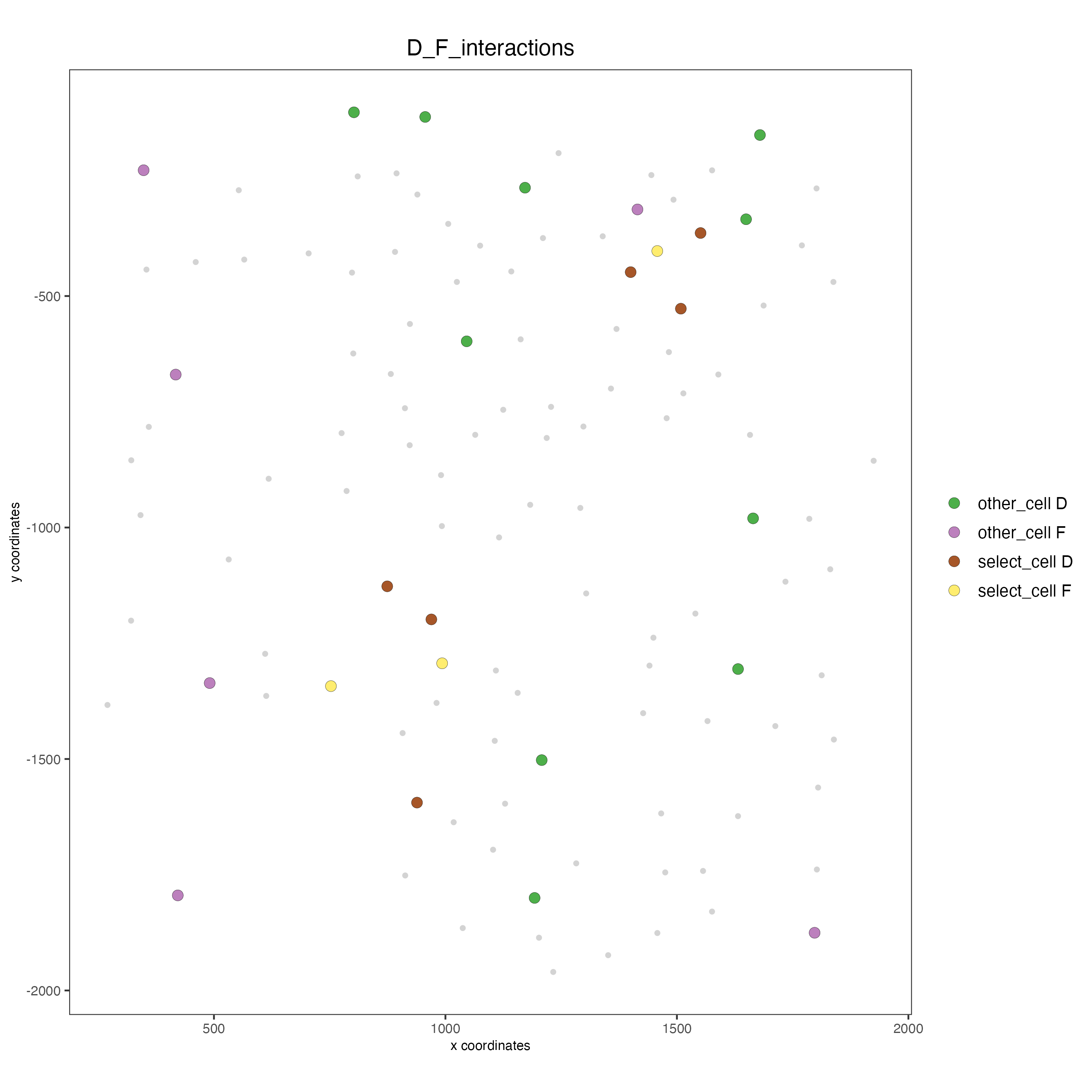
14 Cell neighborhood: Interaction Changed Features
## select top 25 highest expressing genes
gene_metadata <- fDataDT(seqfish_mini)

plot(gene_metadata$nr_cells, gene_metadata$mean_expr)

plot(gene_metadata$nr_cells, gene_metadata$mean_expr_det)

quantile(gene_metadata$mean_expr_det)

high_expressed_genes <- gene_metadata[mean_expr_det > 4]$feat_ID

## identify features (genes) that are associated with proximity to other cell types
ICFscoresHighGenes <- findInteractionChangedFeats(gobject = seqfish_mini,
                                                  selected_feats = high_expressed_genes,
                                                  spatial_network_name = "Delaunay_network",
                                                  cluster_column = "cell_types",
                                                  diff_test = "permutation",
                                                  adjust_method = "fdr",
                                                  nr_permutations = 500,
                                                  do_parallel = TRUE)

## visualize all genes
plotCellProximityFeats(seqfish_mini,
                       icfObject = ICFscoresHighGenes,
                       method = "dotplot")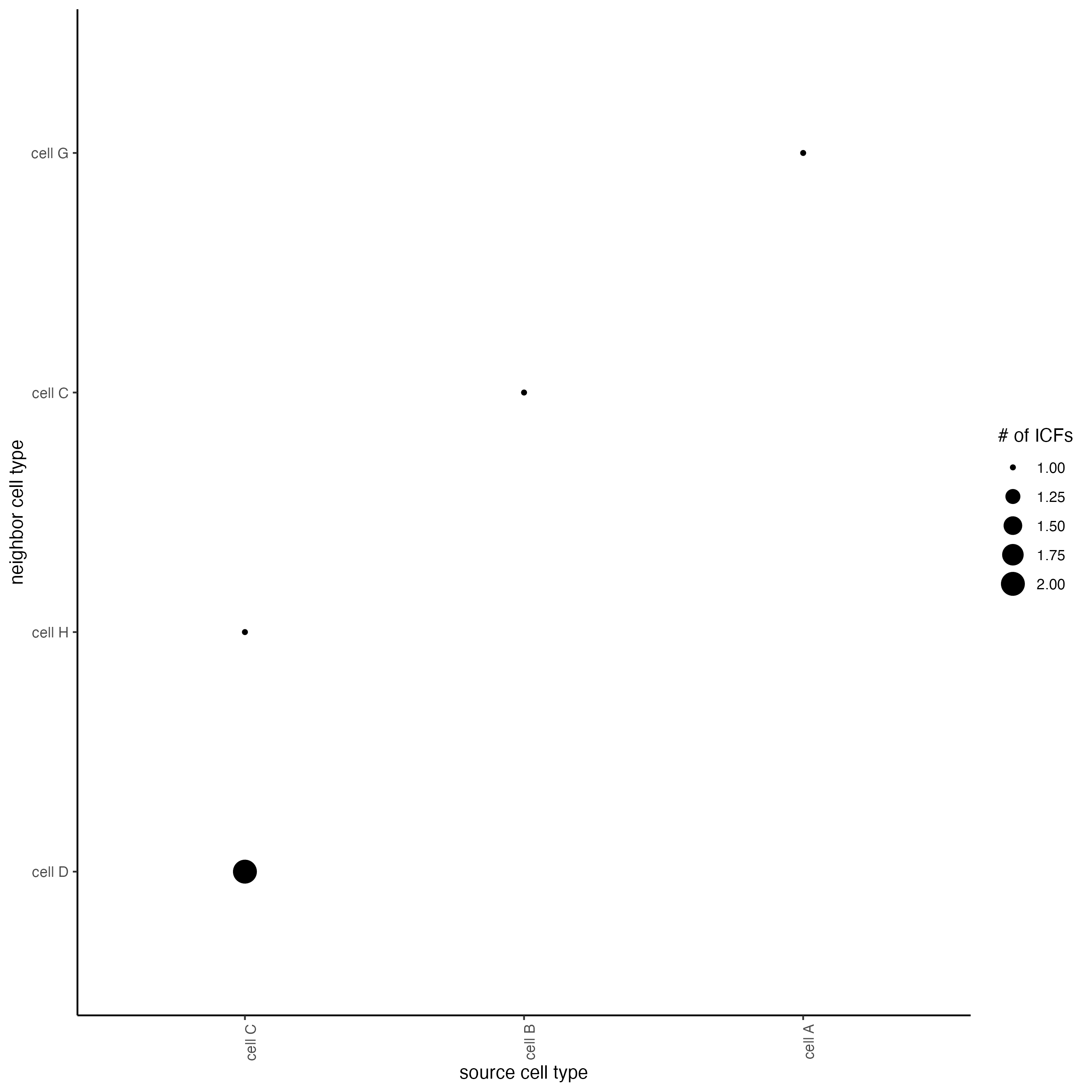
## filter genes
ICFscoresFilt <- filterICF(ICFscoresHighGenes,
                           min_cells = 2,
                           min_int_cells = 2,
                           min_fdr = 0.1,
                           min_spat_diff = 0.1,
                           min_log2_fc = 0.1,
                           min_zscore = 1)

## visualize subset of interaction changed genes (ICGs)
ICF_genes <- c("Cpne2", "Scg3", "Cmtm3", "Cplx1", "Lingo1")
ICF_genes_types <- c("cell E", "cell D", "cell D", "cell G", "cell E")
names(ICF_genes) <- ICF_genes_types

plotICF(gobject = seqfish_mini,
        icfObject = ICFscoresHighGenes,
        source_type = "cell A",
        source_markers = c("Csf1r", "Laptm5"),
        ICF_feats = ICF_genes)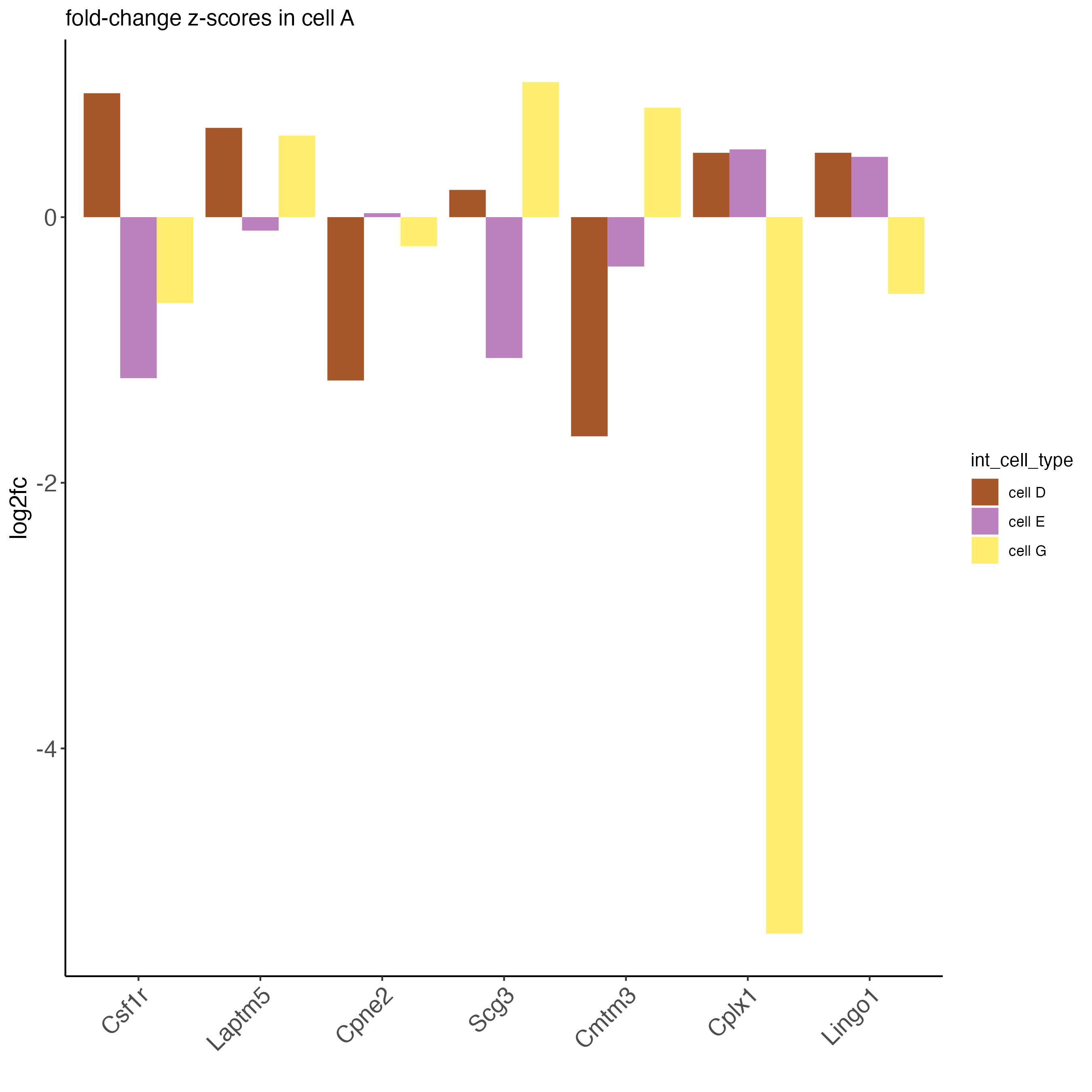
15 Cell Neighborhood: Ligand-Receptor Cell-Cell Communication
LR_data <- data.table::fread(system.file("Mini_datasets/seqfish/Raw/mouse_ligand_receptors.txt",
                                        package = "GiottoData"))

LR_data[, ligand_det := ifelse(mouseLigand %in% seqfish_mini@feat_ID[["rna"]], TRUE, FALSE)]

LR_data[, receptor_det := ifelse(mouseReceptor %in% seqfish_mini@feat_ID[["rna"]], TRUE, FALSE)]

LR_data_det <- LR_data[ligand_det == TRUE & receptor_det == TRUE]

select_ligands <- LR_data_det$mouseLigand

select_receptors <- LR_data_det$mouseReceptor

## get statistical significance of gene pair expression changes based on expression ##
expr_only_scores <- exprCellCellcom(gobject = seqfish_mini,
                                   cluster_column = "cell_types",
                                   random_iter = 50,
                                   feat_set_1 = select_ligands,
                                   feat_set_2 = select_receptors)

## get statistical significance of gene pair expression changes upon cell-cell interaction
spatial_all_scores <- spatCellCellcom(seqfish_mini,
                                     spat_unit = "cell",
                                     feat_type = "rna",
                                     spatial_network_name = "Delaunay_network",
                                     cluster_column = "cell_types",
                                     random_iter = 50,
                                     feat_set_1 = select_ligands,
                                     feat_set_2 = select_receptors,
                                     adjust_method = "fdr",
                                     do_parallel = TRUE,
                                     cores = 4,
                                     verbose = "none")

## * plot communication scores ####
## select top LR ##
selected_spat <- spatial_all_scores[p.adj <= 0.5 & abs(log2fc) > 0.1 & lig_nr >= 2 & rec_nr >= 2]

data.table::setorder(selected_spat, -PI)

top_LR_ints <- unique(selected_spat[order(-abs(PI))]$LR_comb)[1:33]

top_LR_cell_ints <- unique(selected_spat[order(-abs(PI))]$LR_cell_comb)[1:33]

plotCCcomHeatmap(gobject = seqfish_mini,
                 comScores = spatial_all_scores,
                 selected_LR = top_LR_ints,
                 selected_cell_LR = top_LR_cell_ints,
                 show = "LR_expr")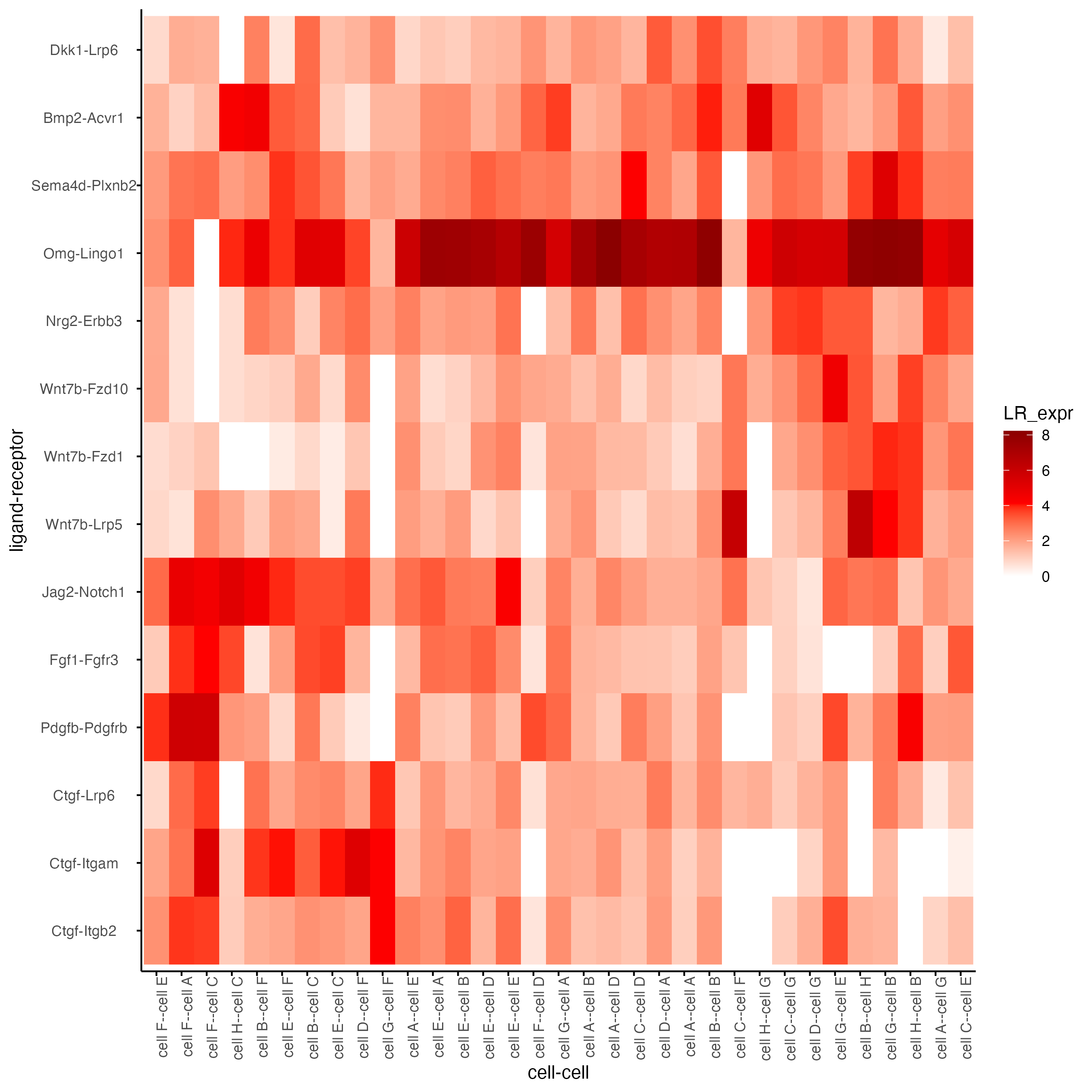
plotCCcomDotplot(gobject = seqfish_mini,
                 comScores = spatial_all_scores,
                 selected_LR = top_LR_ints,
                 selected_cell_LR = top_LR_cell_ints,
                 cluster_on = "PI")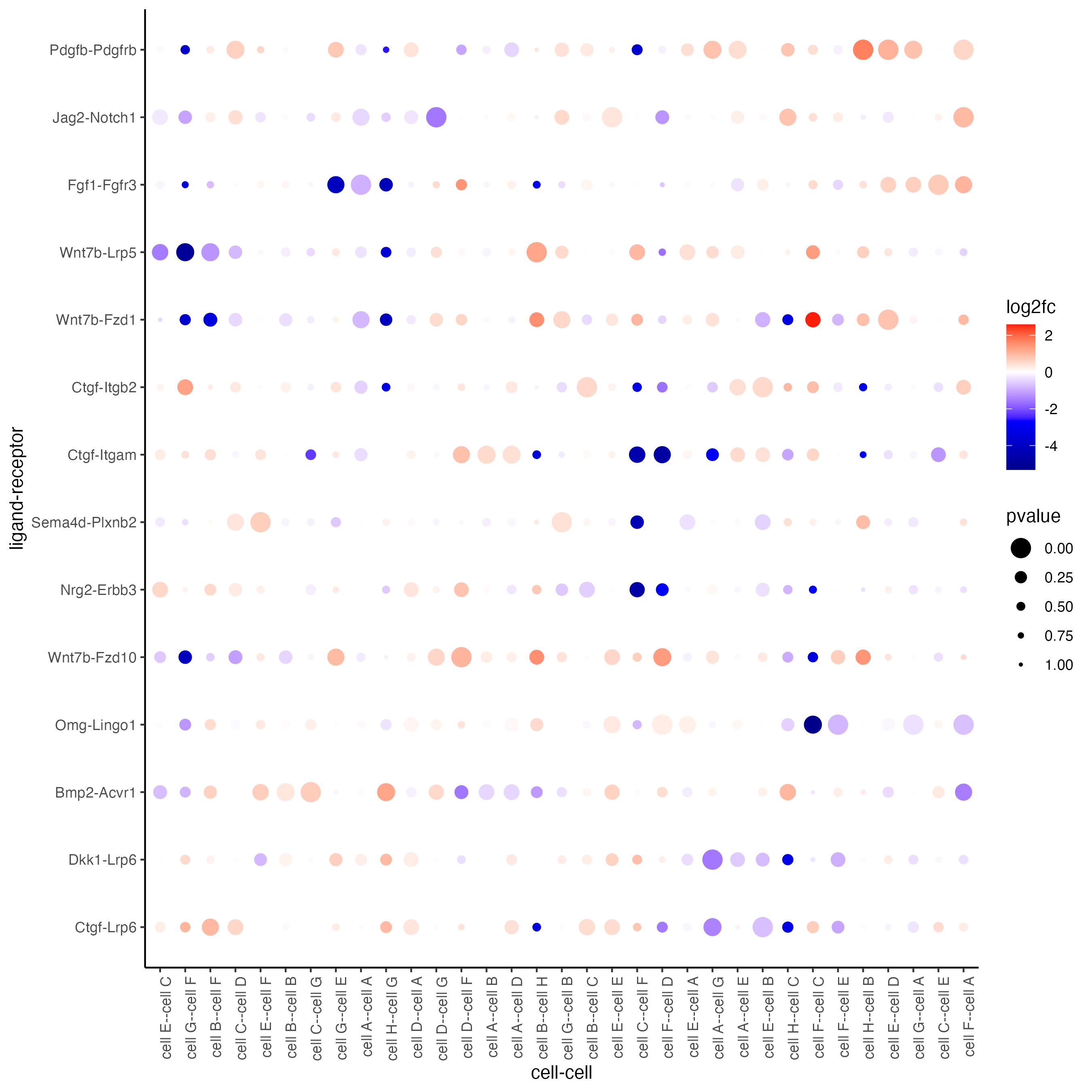
## * spatial vs rank ####
comb_comm <- combCCcom(spatialCC = spatial_all_scores,
                       exprCC = expr_only_scores)

# top differential activity levels for ligand receptor pairs
plotRankSpatvsExpr(gobject = seqfish_mini,
                   comb_comm,
                   expr_rnk_column = "exprPI_rnk",
                   spat_rnk_column = "spatPI_rnk",
                   gradient_midpoint = 10)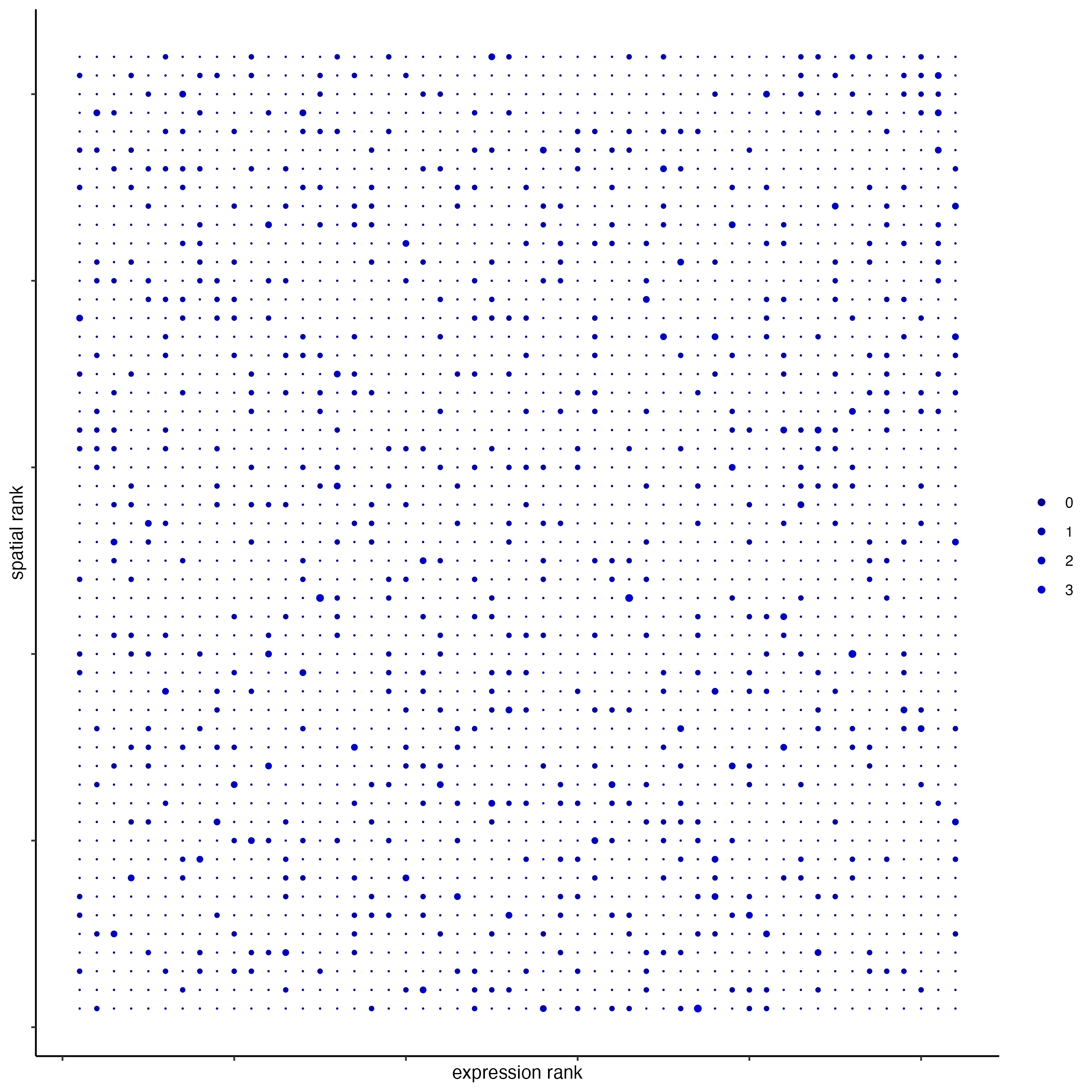
## * recovery ####
## predict maximum differential activity
plotRecovery(gobject = seqfish_mini,
             comb_comm,
             expr_rnk_column = "exprPI_rnk",
             spat_rnk_column = "spatPI_rnk",
             ground_truth = "spatial")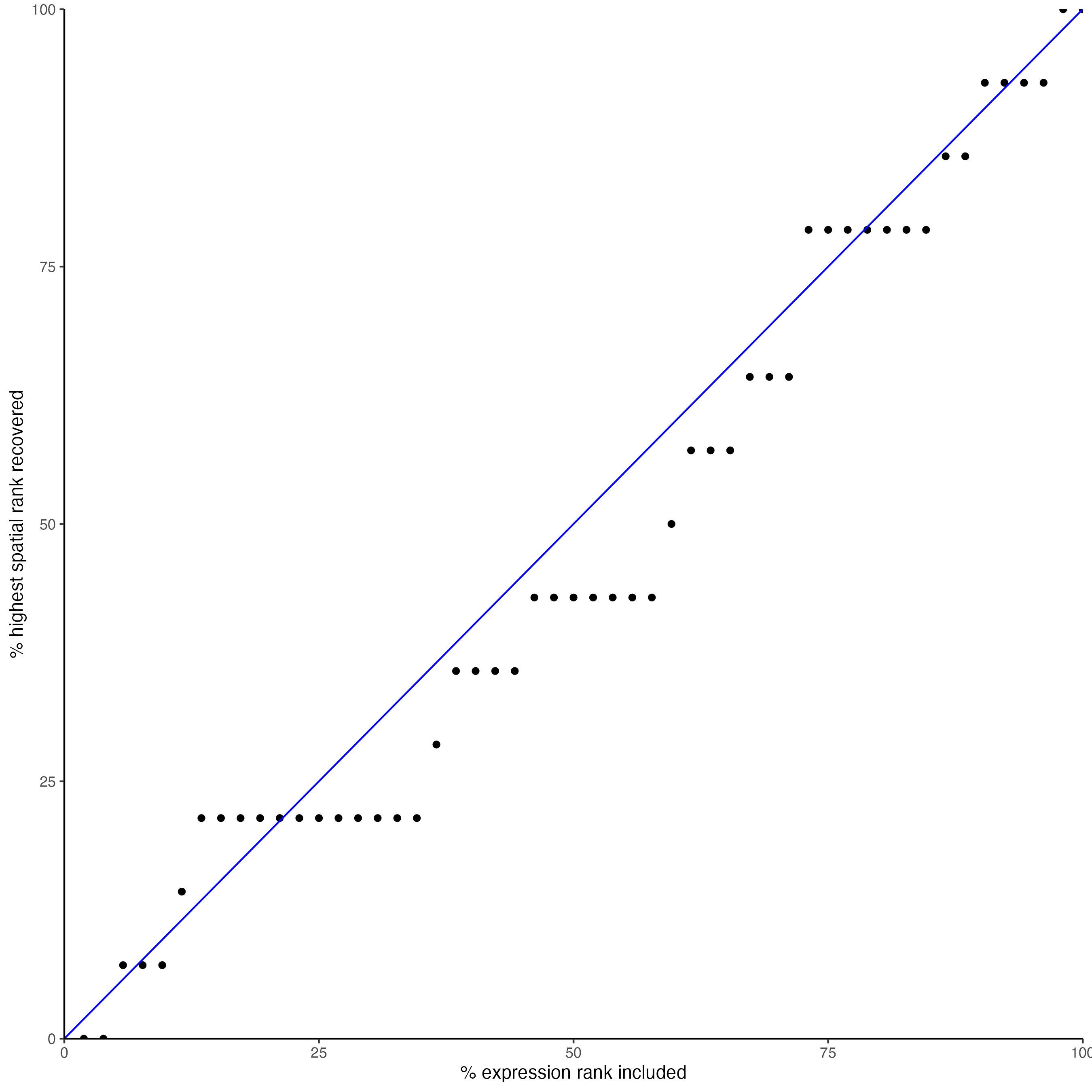
16 Session info
R version 4.3.2 (2023-10-31)
Platform: x86_64-apple-darwin20 (64-bit)
Running under: macOS Sonoma 14.3.1

Matrix products: default
BLAS:   /System/Library/Frameworks/Accelerate.framework/Versions/A/Frameworks/vecLib.framework/Versions/A/libBLAS.dylib
LAPACK: /Library/Frameworks/R.framework/Versions/4.3-x86_64/Resources/lib/libRlapack.dylib;  LAPACK version 3.11.0

locale:
[1] en_US.UTF-8/en_US.UTF-8/en_US.UTF-8/C/en_US.UTF-8/en_US.UTF-8

time zone: America/New_York
tzcode source: internal

attached base packages:
[1] stats     graphics  grDevices utils     datasets  methods   base

other attached packages:
[1] smfishHmrf_0.1     fs_1.6.3           pracma_2.4.4       ggdendro_0.1.23    GiottoData_0.2.7.0
[6] GiottoUtils_0.1.5  Giotto_4.0.2       GiottoClass_0.1.3

loaded via a namespace (and not attached):
  [1] RColorBrewer_1.1-3          rstudioapi_0.15.0           jsonlite_1.8.8
  [4] shape_1.4.6                 magrittr_2.0.3              magick_2.8.2
  [7] farver_2.1.1                rmarkdown_2.25              GlobalOptions_0.1.2
 [10] zlibbioc_1.48.0             ragg_1.2.7                  vctrs_0.6.5
 [13] Cairo_1.6-2                 RCurl_1.98-1.14             terra_1.7-71
 [16] htmltools_0.5.7             S4Arrays_1.2.0              SparseArray_1.2.4
 [19] parallelly_1.36.0           plyr_1.8.9                  igraph_2.0.1.1
 [22] lifecycle_1.0.4             iterators_1.0.14            pkgconfig_2.0.3
 [25] rsvd_1.0.5                  Matrix_1.6-5                R6_2.5.1
 [28] fastmap_1.1.1               GenomeInfoDbData_1.2.11     rbibutils_2.2.16
 [31] MatrixGenerics_1.14.0       future_1.33.1               clue_0.3-65
 [34] digest_0.6.34               colorspace_2.1-0            S4Vectors_0.40.2
 [37] irlba_2.3.5.1               textshaping_0.3.7           GenomicRanges_1.54.1
 [40] beachmat_2.18.0             labeling_0.4.3              progressr_0.14.0
 [43] fansi_1.0.6                 polyclip_1.10-6             abind_1.4-5
 [46] compiler_4.3.2              withr_3.0.0                 doParallel_1.0.17
 [49] backports_1.4.1             BiocParallel_1.36.0         viridis_0.6.5
 [52] ggforce_0.4.1               MASS_7.3-60.0.1             DelayedArray_0.28.0
 [55] rjson_0.2.21                gtools_3.9.5                GiottoVisuals_0.1.4
 [58] tools_4.3.2                 future.apply_1.11.1         glue_1.7.0
 [61] dbscan_1.1-12               grid_4.3.2                  checkmate_2.3.1
 [64] Rtsne_0.17                  cluster_2.1.6               reshape2_1.4.4
 [67] generics_0.1.3              gtable_0.3.4                tidyr_1.3.1
 [70] data.table_1.15.0           tidygraph_1.3.1             BiocSingular_1.18.0
 [73] ScaledMatrix_1.10.0         utf8_1.2.4                  XVector_0.42.0
 [76] BiocGenerics_0.48.1         ggrepel_0.9.5               foreach_1.5.2
 [79] pillar_1.9.0                stringr_1.5.1               limma_3.58.1
 [82] circlize_0.4.15             dplyr_1.1.4                 tweenr_2.0.2
 [85] lattice_0.22-5              FNN_1.1.4                   deldir_2.0-2
 [88] tidyselect_1.2.0            ComplexHeatmap_2.18.0       SingleCellExperiment_1.24.0
 [91] knitr_1.45                  gridExtra_2.3               IRanges_2.36.0
 [94] SummarizedExperiment_1.32.0 stats4_4.3.2                xfun_0.42
 [97] graphlayouts_1.1.0          Biobase_2.62.0              statmod_1.5.0
[100] matrixStats_1.2.0           stringi_1.8.3               yaml_2.3.8
[103] evaluate_0.23               codetools_0.2-19            ggraph_2.1.0
[106] tibble_3.2.1                colorRamp2_0.1.0            cli_3.6.2
[109] uwot_0.1.16                 reticulate_1.35.0           systemfonts_1.0.5
[112] Rdpack_2.6                  munsell_0.5.0               Rcpp_1.0.12
[115] GenomeInfoDb_1.38.6         globals_0.16.2              png_0.1-8
[118] parallel_4.3.2              ggplot2_3.4.4               bitops_1.0-7
[121] listenv_0.9.1               SpatialExperiment_1.12.0    viridisLite_0.4.2
[124] scales_1.3.0                purrr_1.0.2                 crayon_1.5.2
[127] GetoptLong_1.0.5            rlang_1.1.3                 cowplot_1.1.3