Low resolution spatial data typically covers multiple cells making it difficult to delineate the cell contribution to gene expression. Using a process called kriging we can interpolate gene expression and map it to the single cell level from low resolution datasets.
Kriging is a spatial interpolation technique that estimates unknown values at specific locations by weighing nearby known values based on distance and spatial trends. It uses a model to account for both the distance between points and the overall pattern in the data to make accurate predictions. By taking discrete measurement spots, such as those used for visium, we can interpolate gene expression to a finer scale using kriging.
1 Setup and load Giotto
# Ensure Giotto Suite is installed
if(!"Giotto" %in% installed.packages()) {
  pak::pkg_install("drieslab/Giotto")
}

library(Giotto)

# Ensure the Python environment for Giotto has been installed
genv_exists <- checkGiottoEnvironment()

if(!genv_exists){
  # The following command need only be run once to install the Giotto environment
  installGiottoEnvironment()
}
2 Download the dataset
Download the visium brain processed object. You can see more information and the step-by-step analysis in the tutorial.
options(timeout = Inf) # Needed to download large files

data_path <- "/path/to/data/"

destfile <- file.path(data_path, "visium.zip")

download.file("https://zenodo.org/records/13207834/files/01_session5.zip?download=1",
              destfile = destfile)

unzip(destfile, exdir = data_path)
3 Generating a geojson file of nuclei location
Visium datasets require a high resolution H&E or IF image to align spots to. Using these images we can identify individual nuclei and cells to be used for kriging. For the following sections we will need to create a geojson that contains polygon information for the nuclei in the sample. Identifying nuclei is outside the scope of the current tutorial but is required to perform kriging. A tutorial for using qupath can be found here.
Download the nuclei/cell segmentations for this tutorial using the following commands:
destfile <- file.path(data_path, "subcellular_gobject.zip")

download.file("https://zenodo.org/records/13144556/files/Day3_Session6.zip?download=1",
              destfile = destfile)

unzip(destfile, exdir = data_path)
4 Load the visium data
g <- loadGiotto(file.path(data_path, "01_session5/visium_brain_object/"))5 Identifying spatially organized features
We need to identify genes to be used for interpolation. This works best with genes that are spatially distinct. The more genes used for interpolation the longer the analysis will take. See the tutorial for the Detection of spatial genes for more information about this step.
ranktest <- binSpect(g,
    bin_method = "rank",
    calc_hub = TRUE,
    hub_min_int = 5,
    spatial_network_name = "spatial_network"
)

ext_spatial_features <- ranktest[1:15,]$feats
6 Interpolating features
Now we can perform gene expression interpolation. This involves creating a raster image for the gene expression of each of the selected genes. The steps from here can be time consuming and require large amounts of memory.
We will only be analyzing 15 genes to show the process of expression interpolation. For clustering and other analyses more genes are required.
g <- interpolateFeature(g,
                        spat_unit = "cell",
                        feat_type = "rna",
                        ext = ext(g),
                        feats = ext_spatial_features,
                        overwrite = TRUE)
For each gene that we interpolate a raster image is exported based on the gene expression. You can see the list of new images added to the Giotto object running the following command:
7 Adding cell polygons to Giotto object
7.1 Read in the poly information
First we need to read in the geojson file that contains the cell polygons that we’ll interpolate gene expression onto. These will then be added to the Giotto object as a new polygon object. This won’t affect the visium polygons. Both polygons will be stored within the same Giotto object.
# Read in the data
stardist_cell_poly_path <- file.path(data_path, "segmentations/stardist_only_cell_bounds.geojson")

stardist_cell_gpoly <- createGiottoPolygonsFromGeoJSON(GeoJSON = stardist_cell_poly_path,
                                                       name = "stardist_cell",
                                                       calc_centroids = TRUE)

stardist_cell_gpoly <- flip(stardist_cell_gpoly)
7.2 Vizualizing polygons
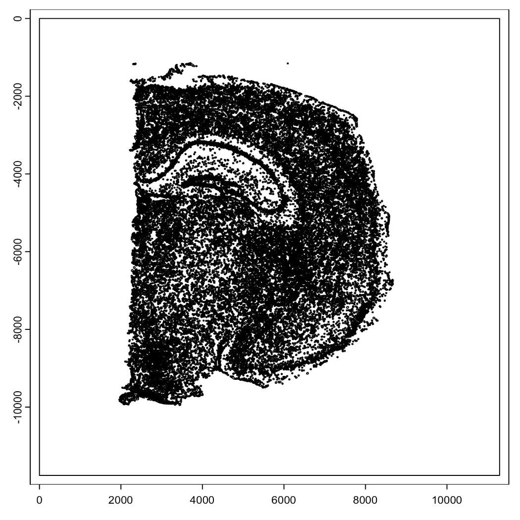
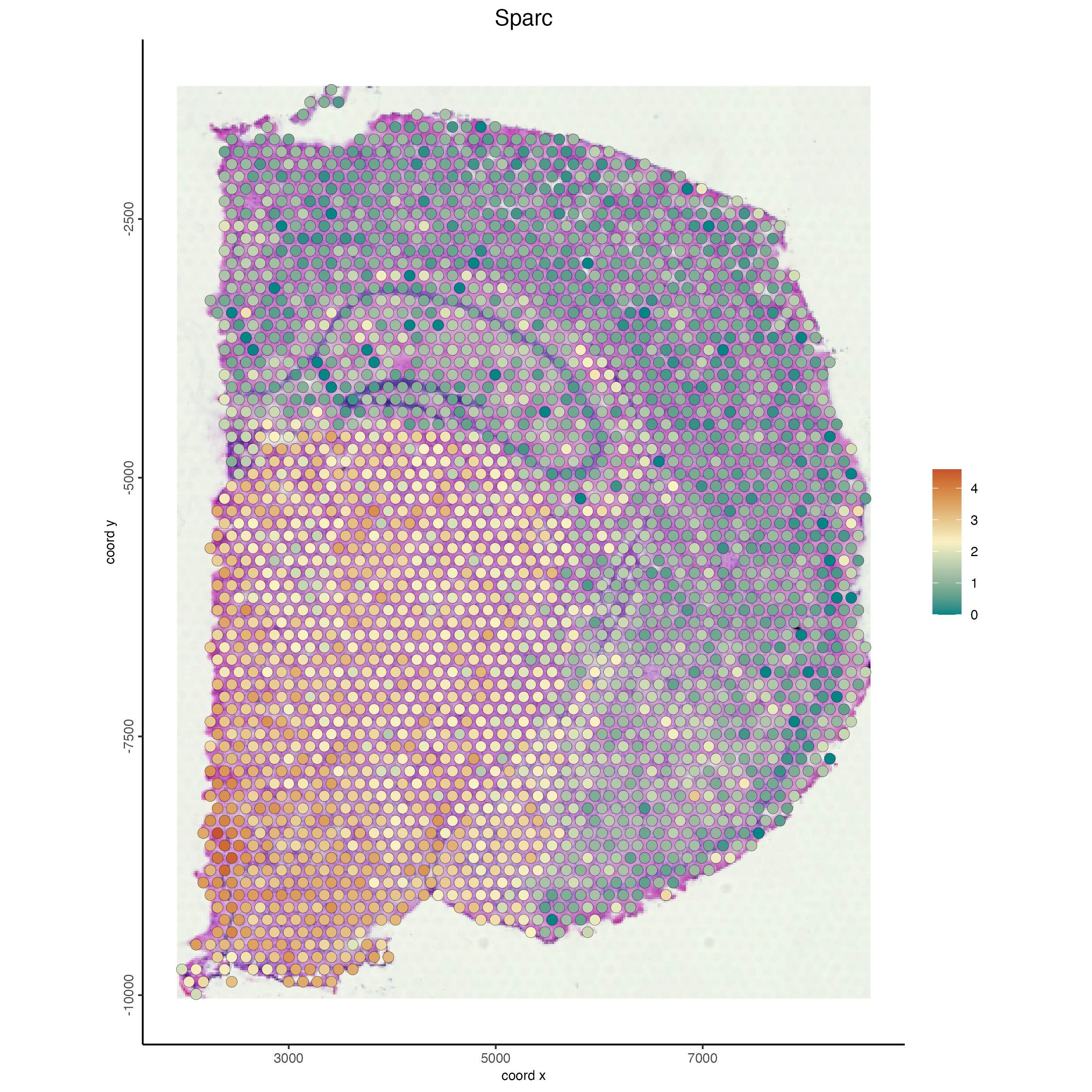
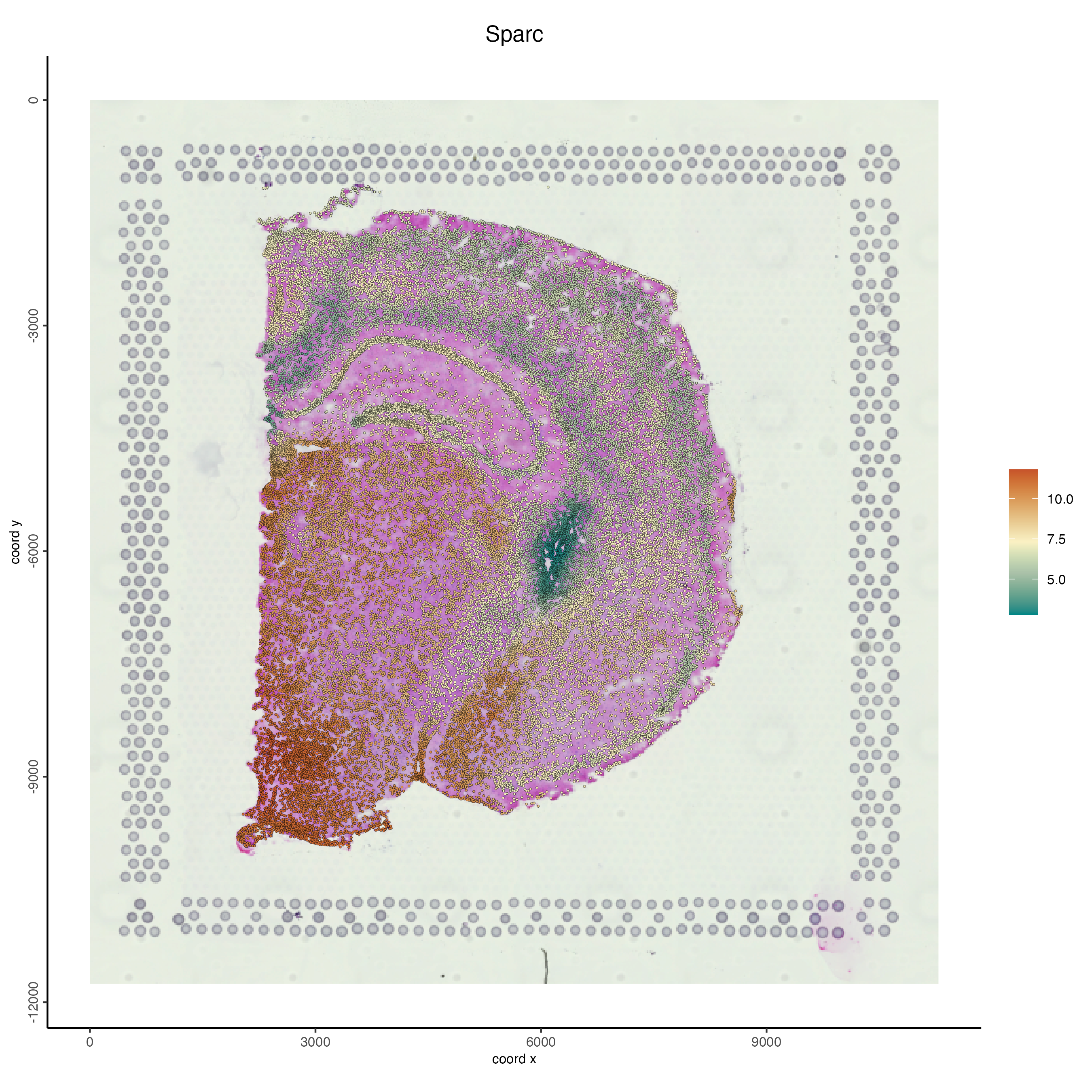
Below we can see a visualization of the polygons for the visium and the nuclei we identified from the H&E image. The visium dataset has 2698 spots compared to the 36694 nuclei we identified. Just using the visium spots we’re therefore losing a lot of the spatial data for individual cells. With the increased number of spots and them directly correlating with the tissue, through the spots alone we are able to better see the actual structure of the mouse brain.
plot(stardist_cell_gpoly, max_poly = 1e6)
7.3 Adding polygons to giotto object
After we add the nuclei polygons we can see that a new polygon name, “stardist_cell” has been added to the gobject.
g <- addGiottoPolygons(g,
                       gpolygons = list("stardist_cell" = stardist_cell_gpoly))
7.4 Check polygon information
We can now see the addition of the new polygons under the name “stardist_cell”. Each of the new polyons is given a unique poly_ID as shown below. Each polygon is also added into same space as the original visium spots, therefore line up with the same image as the visium spots.
getPolygonInfo(g,
               polygon_name = "stardist_cell")
8 Expression overlap
The raster we created above gives the gene expression in a graphical form. We next need to determine how that relates to the nuclei location. To determine that we will calculate the overlap of the rasterized gene expression image to the polygons supplied earlier.
This step also takes more time the more genes that are provided. For large datasets please allow up to multiple hours for these steps to run.
g <- calculateOverlapPolygonImages(gobject = g,
                                   name_overlap = "rna",
                                   spatial_info = "stardist_cell",
                                   image_names = ext_spatial_features)

g <- overlapToMatrix(x = g,
                     poly_info = "stardist_cell",
                     feat_info = "rna",
                     aggr_function = "sum",
                     type = "intensity")
After performing the overlap we now have expression data for each gene provided.
9 Filter and normalization
Now that we have a valid spat unit and gene expression data for each of the provided genes we can now perform the same analyses we used for the regular visium data. Please note that due to the differences in cell number that the values used for the current analysis aren’t identical to the visium analysis.
g <- filterGiotto(gobject = g,
                  spat_unit = "stardist_cell",
                  expression_values = "raw",
                  expression_threshold = 1,
                  feat_det_in_min_cells = 0,
                  min_det_feats_per_cell = 1)

g <- normalizeGiotto(gobject = g,
                     spat_unit = "stardist_cell",
                     scale_cells = FALSE,
                     scale_feats = FALSE,
                     verbose = TRUE)
10 Visualizing gene expression from interpolated expression
Since we have the gene expression information for both the visium and the interpolated gene expression we can visualize gene expression for both from the same Giotto object. We will look at the expression for a genea “Sparc” for both the visium and interpolated data.
spatFeatPlot2D(g,
               spat_unit = "cell",
               gradient_style = "sequential",
               cell_color_gradient = "Geyser",
               feats = "Sparc",
               point_size = 3,
               show_image = TRUE)
spatFeatPlot2D(g,
               spat_unit = "stardist_cell",
               gradient_style = "sequential",
               cell_color_gradient = "Geyser",
               feats = "Sparc",
               point_size = 0.6,
               show_image = TRUE)
11 Session Info
R version 4.4.2 (2024-10-31)
Platform: x86_64-apple-darwin20
Running under: macOS Sequoia 15.0.1

Matrix products: default
BLAS:   /System/Library/Frameworks/Accelerate.framework/Versions/A/Frameworks/vecLib.framework/Versions/A/libBLAS.dylib
LAPACK: /Library/Frameworks/R.framework/Versions/4.4-x86_64/Resources/lib/libRlapack.dylib;  LAPACK version 3.12.0

locale:
[1] en_US.UTF-8/en_US.UTF-8/en_US.UTF-8/C/en_US.UTF-8/en_US.UTF-8

time zone: America/New_York
tzcode source: internal

attached base packages:
[1] stats     graphics  grDevices utils     datasets  methods   base

other attached packages:
[1] data.table_1.16.0 gstat_2.1-2       terra_1.7-78      Giotto_4.1.4
[5] GiottoClass_0.4.3

loaded via a namespace (and not attached):
  [1] colorRamp2_0.1.0            DBI_1.2.3
  [3] rlang_1.1.4                 magrittr_2.0.3
  [5] e1071_1.7-16                GiottoUtils_0.2.0
  [7] matrixStats_1.4.1           compiler_4.4.2
  [9] systemfonts_1.1.0           png_0.1-8
 [11] vctrs_0.6.5                 pkgconfig_2.0.3
 [13] SpatialExperiment_1.14.0    crayon_1.5.3
 [15] fastmap_1.2.0               backports_1.5.0
 [17] magick_2.8.5                XVector_0.44.0
 [19] labeling_0.4.3              utf8_1.2.4
 [21] rmarkdown_2.28              UCSC.utils_1.0.0
 [23] ragg_1.3.3                  purrr_1.0.2
 [25] xfun_0.47                   zlibbioc_1.50.0
 [27] GenomeInfoDb_1.40.1         jsonlite_1.8.9
 [29] DelayedArray_0.30.1         parallel_4.4.2
 [31] R6_2.5.1                    reticulate_1.39.0
 [33] parallelly_1.38.0           GenomicRanges_1.56.1
 [35] scattermore_1.2             Rcpp_1.0.13
 [37] SummarizedExperiment_1.34.0 knitr_1.48
 [39] future.apply_1.11.2         zoo_1.8-12
 [41] IRanges_2.38.1              FNN_1.1.4.1
 [43] Matrix_1.7-1                igraph_2.0.3
 [45] tidyselect_1.2.1            rstudioapi_0.16.0
 [47] abind_1.4-8                 yaml_2.3.10
 [49] codetools_0.2-20            listenv_0.9.1
 [51] lattice_0.22-6              tibble_3.2.1
 [53] intervals_0.15.5            Biobase_2.64.0
 [55] withr_3.0.1                 evaluate_1.0.0
 [57] future_1.34.0               sf_1.0-17
 [59] units_0.8-5                 proxy_0.4-27
 [61] xts_0.14.0                  exactextractr_0.10.0
 [63] pillar_1.9.0                MatrixGenerics_1.16.0
 [65] KernSmooth_2.23-24          checkmate_2.3.2
 [67] stats4_4.4.2                plotly_4.10.4
 [69] generics_0.1.3              sp_2.1-4
 [71] spacetime_1.3-2             S4Vectors_0.42.1
 [73] ggplot2_3.5.1               munsell_0.5.1
 [75] scales_1.3.0                gtools_3.9.5
 [77] globals_0.16.3              class_7.3-22
 [79] glue_1.8.0                  lazyeval_0.2.2
 [81] tools_4.4.2                 GiottoVisuals_0.2.7
 [83] cowplot_1.1.3               grid_4.4.2
 [85] tidyr_1.3.1                 colorspace_2.1-1
 [87] SingleCellExperiment_1.26.0 GenomeInfoDbData_1.2.12
 [89] raster_3.6-26               cli_3.6.3
 [91] textshaping_0.4.0           fansi_1.0.6
 [93] S4Arrays_1.4.1              viridisLite_0.4.2
 [95] dplyr_1.1.4                 gtable_0.3.5
 [97] digest_0.6.37               classInt_0.4-10
 [99] progressr_0.14.0            BiocGenerics_0.50.0
[101] SparseArray_1.4.8           ggrepel_0.9.6
[103] farver_2.1.2                rjson_0.2.23
[105] htmlwidgets_1.6.4           htmltools_0.5.8.1
[107] lifecycle_1.0.4             httr_1.4.7