Interactive region selection on large datasets
Source:vignettes/interactive_selection_cosmx.Rmd
interactive_selection_cosmx.RmdWhile the interactive region selection using the Shiny app is very user-friendly, it doesn’t offer the best performance when handling big datasets.
We have created a function that facilitates the interaction with the vitessceR package for interactive visualization of processed large datasets.
1 Set up the Giotto enviroment
# Ensure Giotto Suite is installed.
if(!"Giotto" %in% installed.packages()) {
  pak::pkg_install("drieslab/Giotto")
}

library(Giotto)

# Ensure the Python environment for Giotto has been installed.
genv_exists <- checkGiottoEnvironment()
if(!genv_exists){
  # The following command need only be run once to install the Giotto environment.
  installGiottoEnvironment()
}
2 Install the vitessceR package
pak::pkg_install("vitessce/vitessceR")3 Dataset explanation
For this tutorial, we will use the Nanostring CosMx Subcellular Lung Cancer processed Giotto object.
4 Load the Giotto object
If you have the object already in your R environment, you can skip
this step. If you exported it to a folder using the
saveGiotto() function, then run the following command:
giotto_object <- loadGiotto("cosmx_object/")5 Export the Giotto object to a local Anndata-Zarr folder
By default, the function giottoToAnndataZarr() will look for the “cell” spatial unit and “rna” feature type, but you can specify the spat_unit and feat_type arguments, as well as the expression values to use.
In addition, you need to specify the path or name for creating a new folder that will store the Anndata-Zarr information.
giottoToAnndataZarr(giotto_object,
                    output_path = "cosmx_anndata_zarr",
                    expression = "normalized")
6 Create the vitessceR object
To create the vitessceR object, you need to provide the paths for the metadata information that you want to load from your Anndata-Zarr folder. We suggest to explore the subfolders obs (for cell metadata), var (for feature metadata), and obsm (for spatial and dimension reduction data).
library(vitessceR)

w <- AnnDataWrapper$new(
  adata_path = "cosmx_anndata_zarr",
  obs_feature_matrix_path = "X",
  obs_set_paths = c("obs/leiden_clus", "obs/cell_types"),
  obs_set_names = c("Leiden clusters", "Cell types"),
  obs_locations_path = "obsm/spatial",
  obs_embedding_paths = c("obsm/spatial", "obsm/pca", "obsm/tsne", "obsm/umap"),
  obs_embedding_names = c("Spatial", "PCA",  "t-SNE", "UMAP"),
  feature_labels_path = "var/feat_ID",
  obs_labels_paths = "obs/cell_ID",
  obs_labels_names = "cell_ID",
)
7 Create the vitessceR schema
Here we will create the base of the schema using the previous object, then we will add the components to generate interactive plots.
vc <- VitessceConfig$new(schema_version = "1.0.16", name = "My config")
dataset <- vc$add_dataset("My dataset")$add_object(w)
cluster_sets <- vc$add_view(dataset, Component$OBS_SETS)
features <- vc$add_view(dataset, Component$FEATURE_LIST)
scatterplot_spatial <- vc$add_view(dataset, Component$SCATTERPLOT, mapping = "Spatial")
scatterplot_pca <- vc$add_view(dataset, Component$SCATTERPLOT, mapping = "PCA")
scatterplot_umap <- vc$add_view(dataset, Component$SCATTERPLOT, mapping = "UMAP")
scatterplot_tsne <- vc$add_view(dataset, Component$SCATTERPLOT, mapping = "t-SNE")
desc <- vc$add_view(dataset, Component$DESCRIPTION)
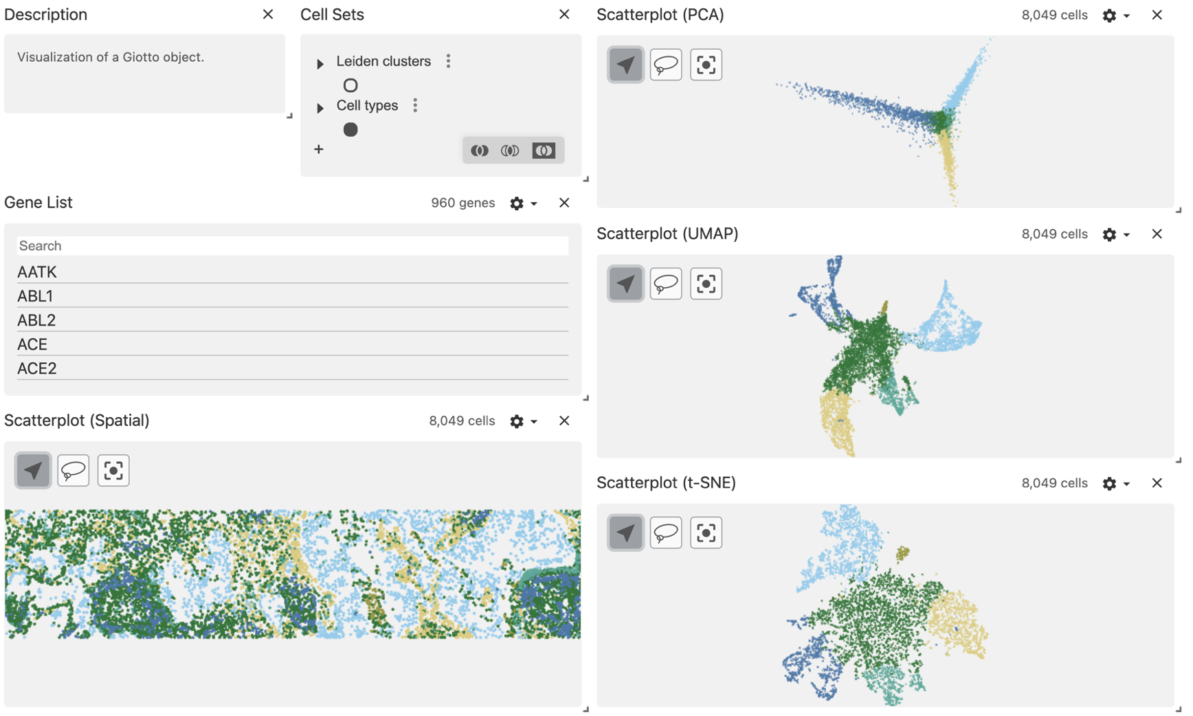
desc <- desc$set_props(description = "Visualization of a Giotto object.")8 Create the layout
You can create multi-column layout and add more compartments using the horizontal (hconcat) or vertical (vconcat) sections.
vc$layout(
  hconcat(
    vconcat(
      hconcat(desc, cluster_sets),
      features,
      scatterplot_spatial
      ),
    vconcat(
      scatterplot_pca,
      scatterplot_umap,
      scatterplot_tsne)
  )
)
10 Select the regions of interest
Use the lasso tool to select a region of interest.
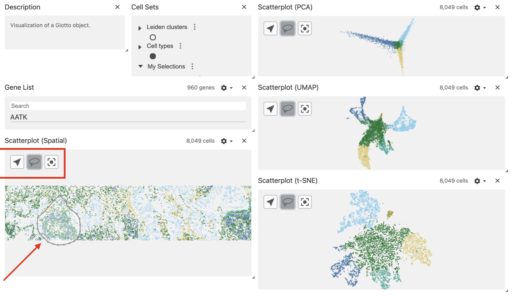
After drawing the selection, the area will be highlighted and the corresponding cells will be mapped and highlighted in the dimension reduction plots.
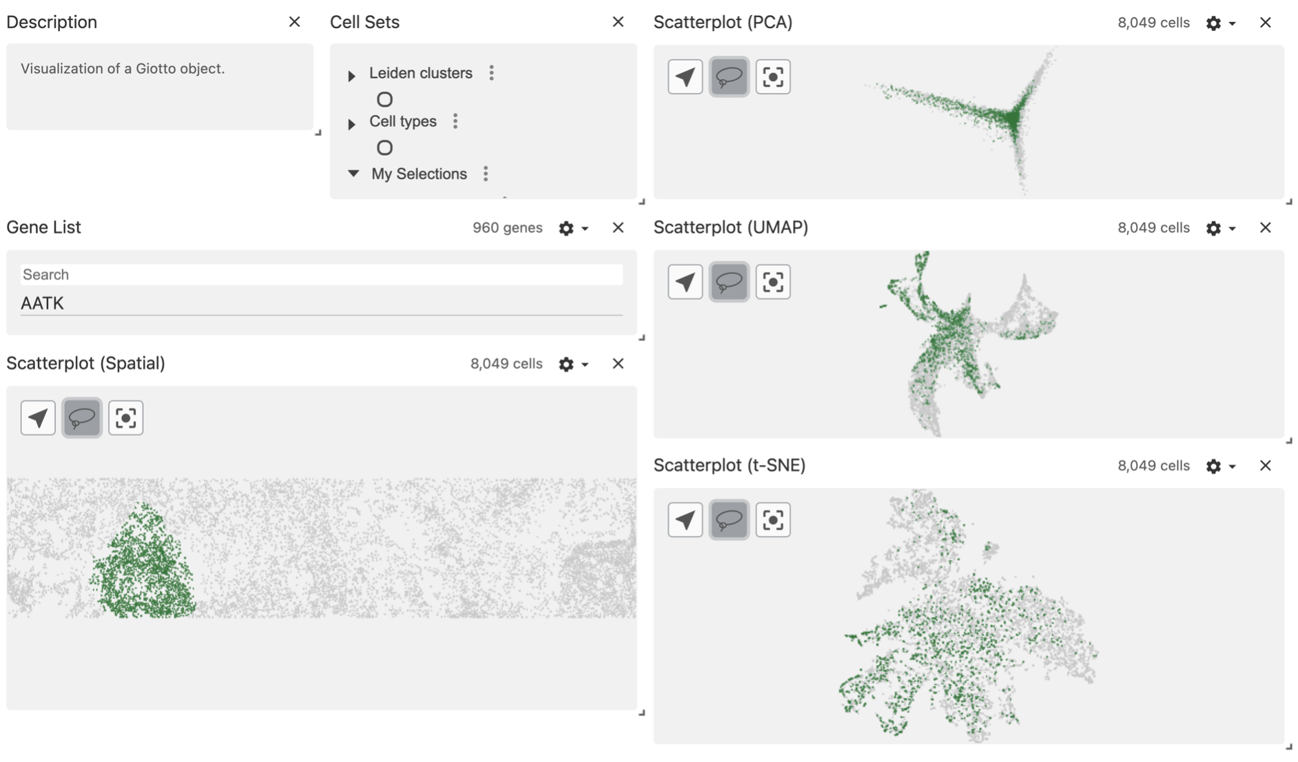
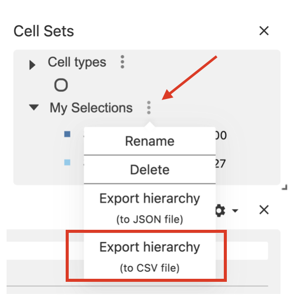
You can see your selected regions in the Cell Sets panel, under the My Selections group.
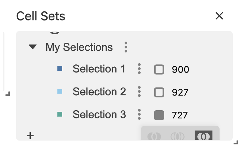
11 Export your selected regions
When you have finished selecting the regions of interest, click on the dots menu and select the option Export hierarchy to csv.
12 Add the selected regions to the Giotto object
12.1 Read the selections file
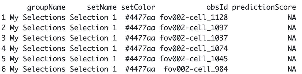
Use the cell_IDs to add their corresponding spatial coordinates.
spatial_locs <- getSpatialLocations(giotto_object,
                                    output = "data.table")

my_selections <- merge(my_selections, spatial_locs)
my_selections <- my_selections[order(my_selections$setName),]
12.2 Create a Giotto polygon object
We must transform the data.frame with coordinates into a Giotto polygon object.
my_giotto_polygons <- createGiottoPolygonsFromDfr(my_selections[, c("sdimx", "sdimy", "setName")],
                                                  name = "selections",
                                                  calc_centroids = TRUE)

giotto_object <- addGiottoPolygons(gobject = giotto_object,
                                   gpolygons = list(my_giotto_polygons))
12.3 Add the cells within the polygons to the Giotto object
giotto_object <- addPolygonCells(giotto_object,
                                 polygon_name = "selections")
Let’s see how it looks like now the cell_metadata
pDataDT(giotto_object)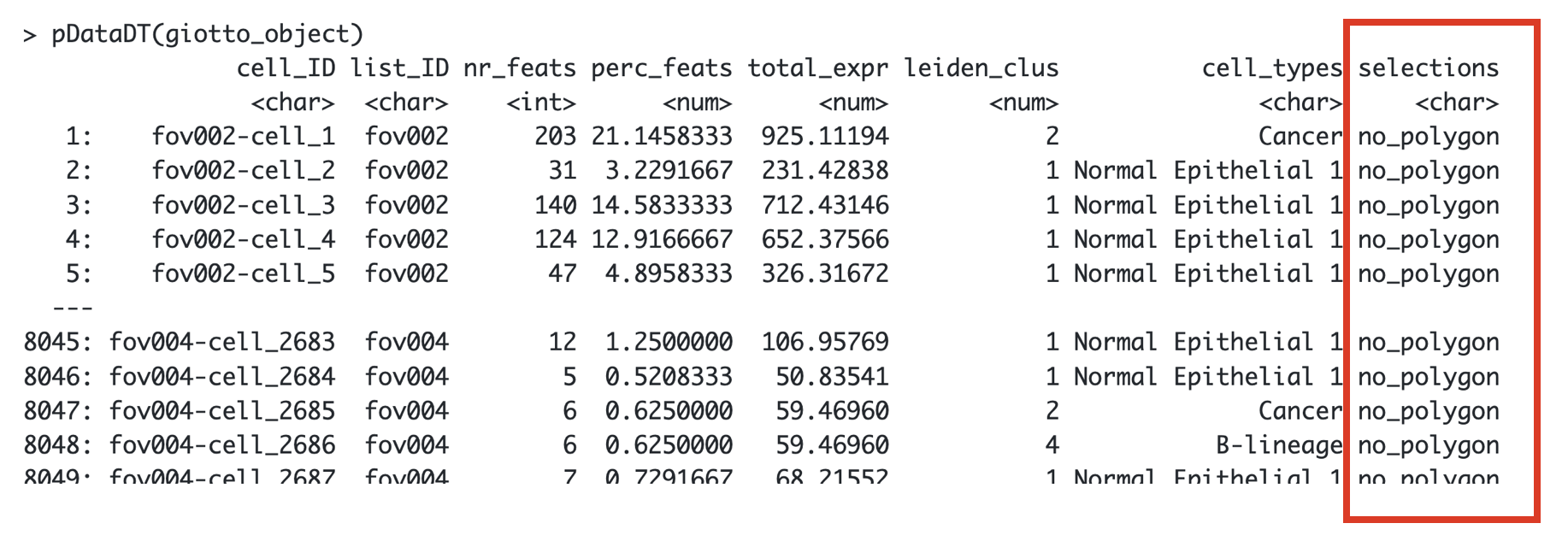
13 Downstream analysis
13.1 Extract the cells within each selected region
By default, the function will retrieve the cells located within all
the selected regions. You can use the argument polygons to
specify what Selection you want to get, e.g “Selection 1”.
getCellsFromPolygon(giotto_object,
                    polygon_name = "selections")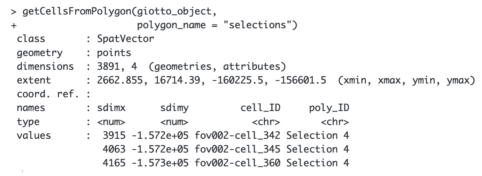
13.2 Compare the cell types between regions
compareCellAbundance(giotto_object,
                     cell_type_column = "cell_types")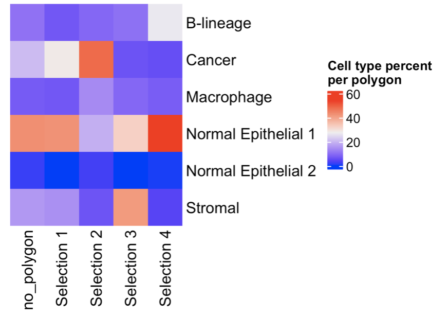
13.3 Compare the gene expression between regions
You can provide a list of genes
comparePolygonExpression(giotto_object,
                         selected_feats = c("KRT19", "SERPINA1", "TYK2"))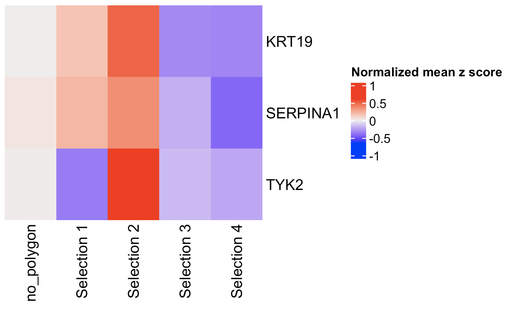
Or you can calculate the top expressed genes per region and then plot them.
markers_scran <- findMarkers_one_vs_all(gobject = giotto_object,
                                        method = "scran",
                                        expression_values = "normalized",
                                        cluster_column = "selections")

topgenes_scran <- markers_scran[, head(.SD, 2), by = "cluster"]$feats

comparePolygonExpression(giotto_object,
                         selected_feats = topgenes_scran)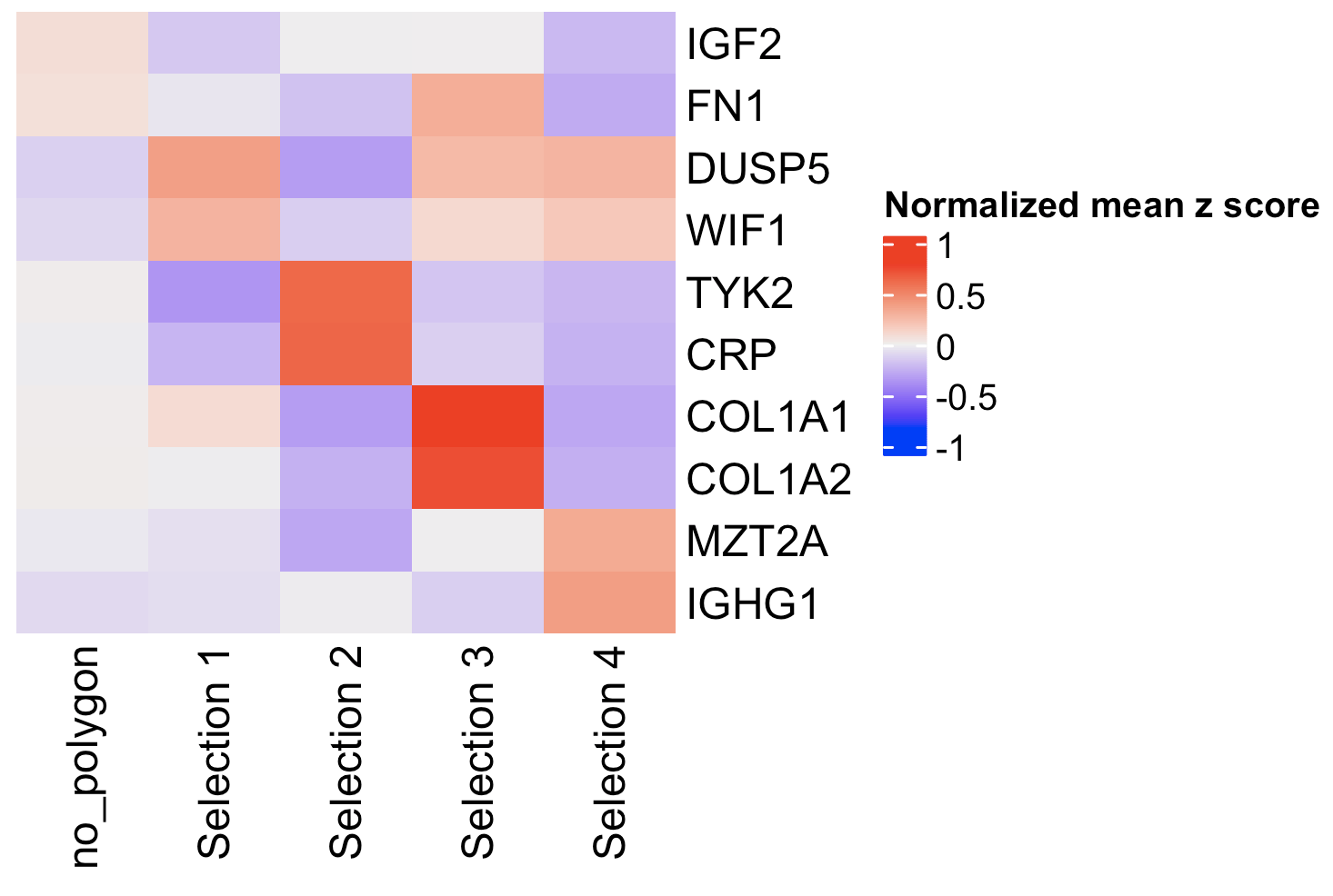
13.4 Plot again the selected regions
Use the ‘selections’ column in the metadata table to color the cells with their corresponding Selection ID.
spatPlot2D(giotto_object,
           cell_color = "selections",
           point_size = 1)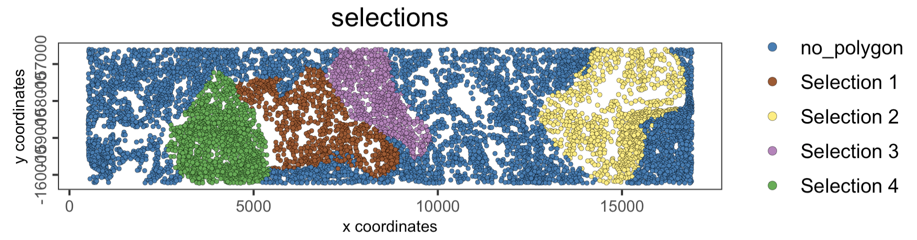
14 Session info
R version 4.4.1 (2024-06-14)
Platform: x86_64-apple-darwin20
Running under: macOS 15.0

Matrix products: default
BLAS:   /System/Library/Frameworks/Accelerate.framework/Versions/A/Frameworks/vecLib.framework/Versions/A/libBLAS.dylib
LAPACK: /Library/Frameworks/R.framework/Versions/4.4-x86_64/Resources/lib/libRlapack.dylib;  LAPACK version 3.12.0

locale:
[1] en_US.UTF-8/en_US.UTF-8/en_US.UTF-8/C/en_US.UTF-8/en_US.UTF-8

time zone: America/New_York
tzcode source: internal

attached base packages:
[1] stats     graphics  grDevices utils     datasets  methods   base

other attached packages:
[1] vitessceR_0.99.0  Giotto_4.1.3      GiottoClass_0.4.0

loaded via a namespace (and not attached):
  [1] RColorBrewer_1.1-3          rstudioapi_0.16.0
  [3] jsonlite_1.8.8              shape_1.4.6.1
  [5] magrittr_2.0.3              magick_2.8.4
  [7] farver_2.1.2                GlobalOptions_0.1.2
  [9] zlibbioc_1.50.0             ragg_1.3.2
 [11] vctrs_0.6.5                 DelayedMatrixStats_1.26.0
 [13] Cairo_1.6-2                 GiottoUtils_0.1.12
 [15] terra_1.7-78                htmltools_0.5.8.1
 [17] S4Arrays_1.4.1              BiocNeighbors_1.22.0
 [19] SparseArray_1.4.8           parallelly_1.38.0
 [21] htmlwidgets_1.6.4           basilisk_1.16.0
 [23] desc_1.4.3                  plotly_4.10.4
 [25] igraph_2.0.3                lifecycle_1.0.4
 [27] iterators_1.0.14            pkgconfig_2.0.3
 [29] rsvd_1.0.5                  Matrix_1.7-0
 [31] R6_2.5.1                    fastmap_1.2.0
 [33] GenomeInfoDbData_1.2.12     MatrixGenerics_1.16.0
 [35] future_1.34.0               clue_0.3-65
 [37] digest_0.6.37               colorspace_2.1-1
 [39] S4Vectors_0.42.1            rprojroot_2.0.4
 [41] dqrng_0.4.1                 irlba_2.3.5.1
 [43] textshaping_0.4.0           GenomicRanges_1.56.1
 [45] beachmat_2.20.0             filelock_1.0.3
 [47] labeling_0.4.3              progressr_0.14.0
 [49] fansi_1.0.6                 httr_1.4.7
 [51] abind_1.4-5                 compiler_4.4.1
 [53] here_1.0.1                  withr_3.0.1
 [55] doParallel_1.0.17           backports_1.5.0
 [57] BiocParallel_1.38.0         webutils_1.2.1
 [59] R.utils_2.12.3              DelayedArray_0.30.1
 [61] bluster_1.14.0              rjson_0.2.22
 [63] gtools_3.9.5                GiottoVisuals_0.2.5
 [65] tools_4.4.1                 httpuv_1.6.15
 [67] R.oo_1.26.0                 glue_1.7.0
 [69] dbscan_1.2-0                promises_1.3.0
 [71] grid_4.4.1                  checkmate_2.3.2
 [73] Rtsne_0.17                  cluster_2.1.6
 [75] generics_0.1.3              plumber_1.2.2
 [77] gtable_0.3.5                R.methodsS3_1.8.2
 [79] tidyr_1.3.1                 data.table_1.16.0
 [81] metapod_1.12.0              ScaledMatrix_1.12.0
 [83] BiocSingular_1.20.0         sp_2.1-4
 [85] utf8_1.2.4                  XVector_0.44.0
 [87] BiocGenerics_0.50.0         RcppAnnoy_0.0.22
 [89] ggrepel_0.9.6               foreach_1.5.2
 [91] pillar_1.9.0                limma_3.60.4
 [93] later_1.3.2                 circlize_0.4.16
 [95] dplyr_1.1.4                 lattice_0.22-6
 [97] swagger_5.17.14.1           deldir_2.0-4
 [99] tidyselect_1.2.1            locfit_1.5-9.10
[101] ComplexHeatmap_2.20.0       SingleCellExperiment_1.26.0
[103] scuttle_1.14.0              IRanges_2.38.1
[105] edgeR_4.2.1                 SummarizedExperiment_1.34.0
[107] scattermore_1.2             stats4_4.4.1
[109] Biobase_2.64.0              statmod_1.5.0
[111] matrixStats_1.4.1           stringi_1.8.4
[113] UCSC.utils_1.0.0            lazyeval_0.2.2
[115] yaml_2.3.10                 codetools_0.2-20
[117] GiottoData_0.2.13           tibble_3.2.1
[119] colorRamp2_0.1.0            cli_3.6.3
[121] reticulate_1.39.0           systemfonts_1.1.0
[123] munsell_0.5.1               Rcpp_1.0.13
[125] GenomeInfoDb_1.40.1         globals_0.16.3
[127] dir.expiry_1.12.0           png_0.1-8
[129] parallel_4.4.1              ggplot2_3.5.1
[131] basilisk.utils_1.16.0       scran_1.32.0
[133] sparseMatrixStats_1.16.0    listenv_0.9.1
[135] SpatialExperiment_1.14.0    viridisLite_0.4.2
[137] scales_1.3.0                purrr_1.0.2
[139] crayon_1.5.3                GetoptLong_1.0.5
[141] rlang_1.1.4                 cowplot_1.1.3