Nanostring CosMx Subcellular Lung Cancer
Source:vignettes/nanostring_cosmx_lung_cancer.Rmd
nanostring_cosmx_lung_cancer.Rmd1 Dataset explanation
This example uses subcellular data from Nanostring”s CosMx Spatial Molecular Imager. This publicly available dataset is from an FFPE sample of non-small-cell lung cancer (NSCLC). This example works with Lung12.
# Ensure Giotto Suite is installed.
if(!"Giotto" %in% installed.packages()) {
  pak::pkg_install("drieslab/Giotto")
}

# Ensure the Python environment for Giotto has been installed.
genv_exists <- Giotto::checkGiottoEnvironment()
if(!genv_exists){
  # The following command need only be run once to install the Giotto environment.
  Giotto::installGiottoEnvironment()
}
2 Setup
library(Giotto)

# set working directory
results_folder <- "/path/to/results/"

# Optional: Specify a path to a Python executable within a conda or miniconda
# environment. If set to NULL (default), the Python executable within the previously
# installed Giotto environment will be used.
python_path <- NULL # alternatively, "/local/python/path/python" if desired.

## Set object behavior
# by directly saving plots, but not rendering them you will save a lot of time
instrs <- createGiottoInstructions(
    save_dir = results_folder,
    save_plot = TRUE,
    show_plot = FALSE,
    return_plot = FALSE,
    python_path = python_path
)
3 Create the Giotto object using the import utility
## provide path to nanostring folder
data_path <- "/path/to/data/"

## create giotto cosmx object
cosmx <- createGiottoCosMxObject(
    cosmx_dir = data_path,
    version = "legacy", # set to this for legacy NSCLC dataset
    FOVs = seq_len(28), # defaults to all FOVs
    load_expression = FALSE, # defaults to FALSE (see feature aggregation step below)
    instructions = instrs
)
CosMx data is very FOV-based, and a column called fov is
included in the cell metadata.
4 Visualize Cells and Genes of Interest
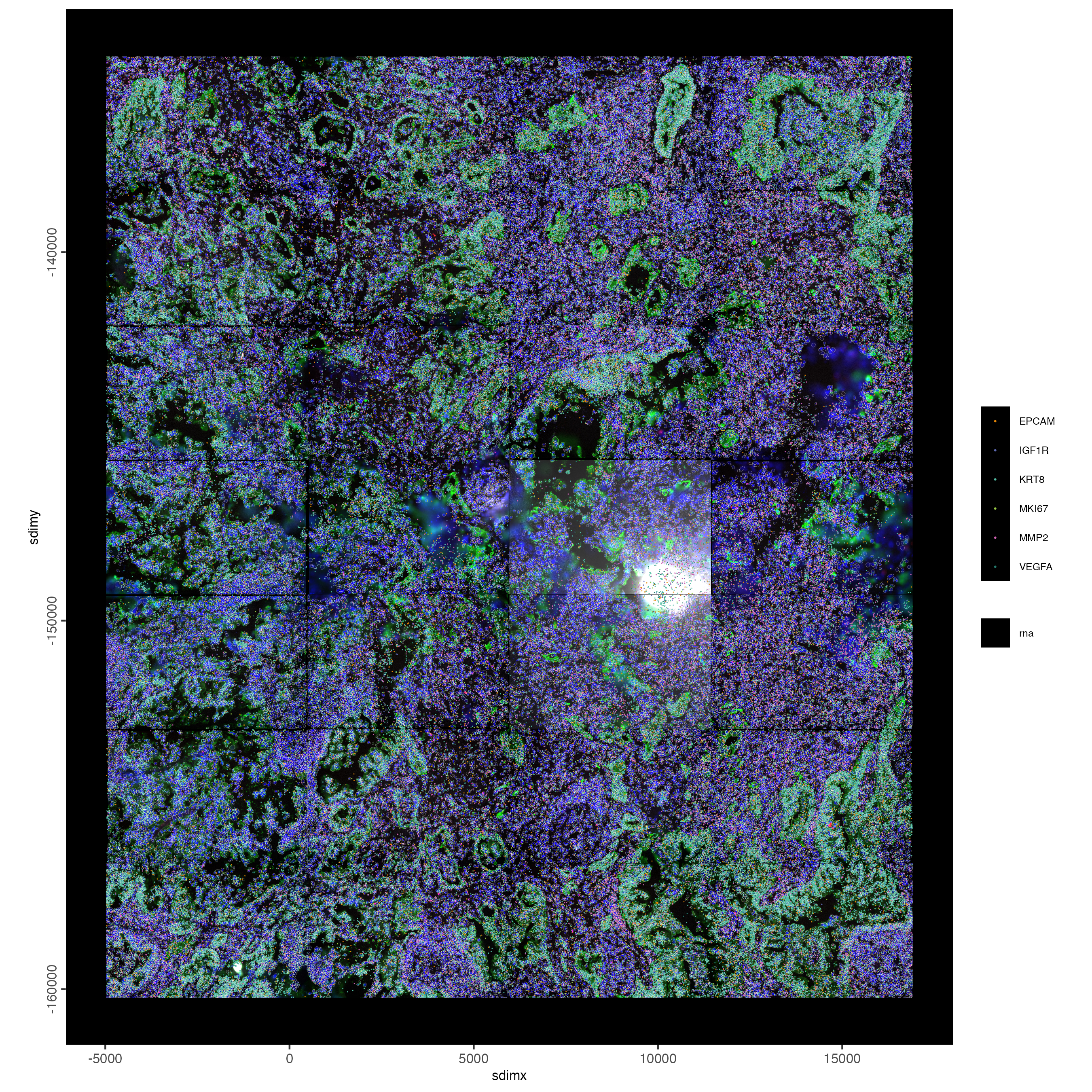
When plotting subcellular data, Giotto uses the
spatInSituPlot functions. Spatial plots showing the feature
points and polygons are plotted using
spatInSituPlotPoints().
showGiottoImageNames(cosmx)
# Set up vector of image names
id_set <- seq_len(28) # there are 28 FOVs here
image_names <- sprintf("composite_fov%03d", id_set)
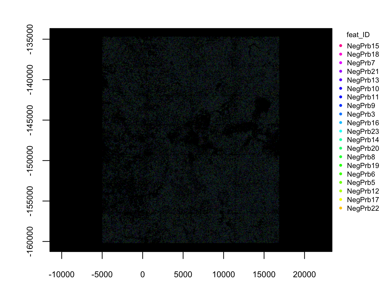
spatInSituPlotPoints(cosmx,
show_image = TRUE,
image_name = image_names,
feats = list("rna" = c(
"MMP2", "VEGFA", "IGF1R",
"MKI67", "EPCAM", "KRT8")
),
feats_color_code = getColors("Vivid", 10),
spat_unit = "cell",
point_size = 0.01,
use_overlap = FALSE,
polygon_alpha = 0,
polygon_color = "white",
polygon_line_size = 0.03,
save_param = list(
save_name = "1_poly_plot"
)
)
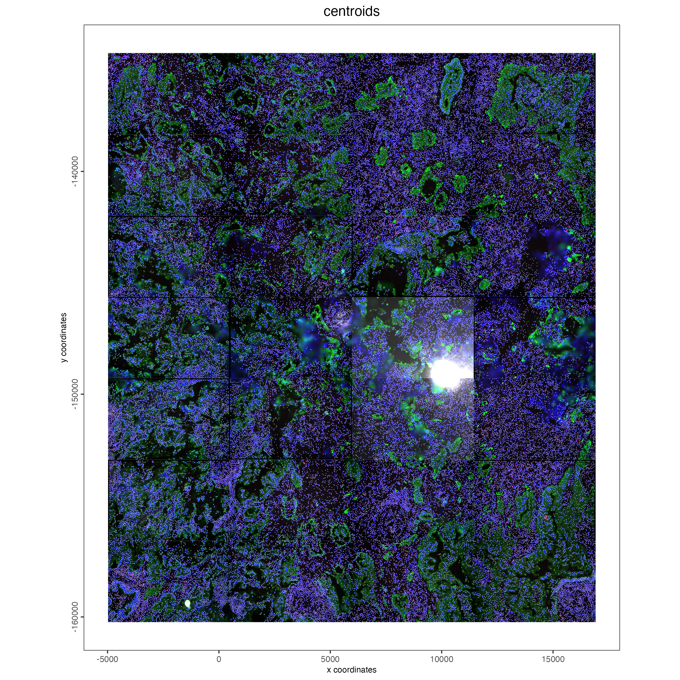
4.1 Visualize Cell Centroids
spatPlot2D(cosmx,
    image_name = image_names,
    show_image = TRUE,
    point_border_stroke = 0,
    cell_color = "white",
    point_size = 0.3,
    point_alpha = 0.8,
    title = "centroids",
    save_param = list(
        save_name = "2_centroids_plot"
    )
)
5 Aggregate subcellular features
For more information on feature aggregation: link
To generate a cell by feature matrix, Giotto performs feature detection aggregation based on the cell polygons. This workflow is recommended over loading the matrix provided in the outputs.
If directly loading the expression info in the outputs is desired,
set load_expression (and also load_cellmeta)
to TRUE when creating the object with
createGiottoCosMxObject()
# Find the feature points overlapped by polygons. This overlap information is then
# returned to the relevant giottoPolygon object"s overlaps slot.
cosmx <- calculateOverlapRaster(cosmx, feat_info = "rna")
cosmx <- calculateOverlapRaster(cosmx, feat_info = "negprobes")
# Convert the overlap information into a cell by feature expression matrix which
# is then stored in the Giotto object"s expression slot
cosmx <- overlapToMatrix(cosmx, feat_info = "rna")
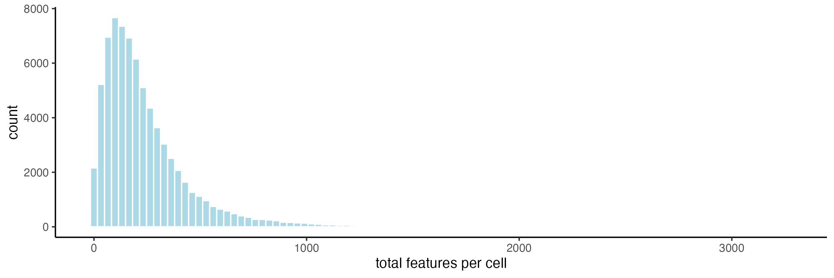
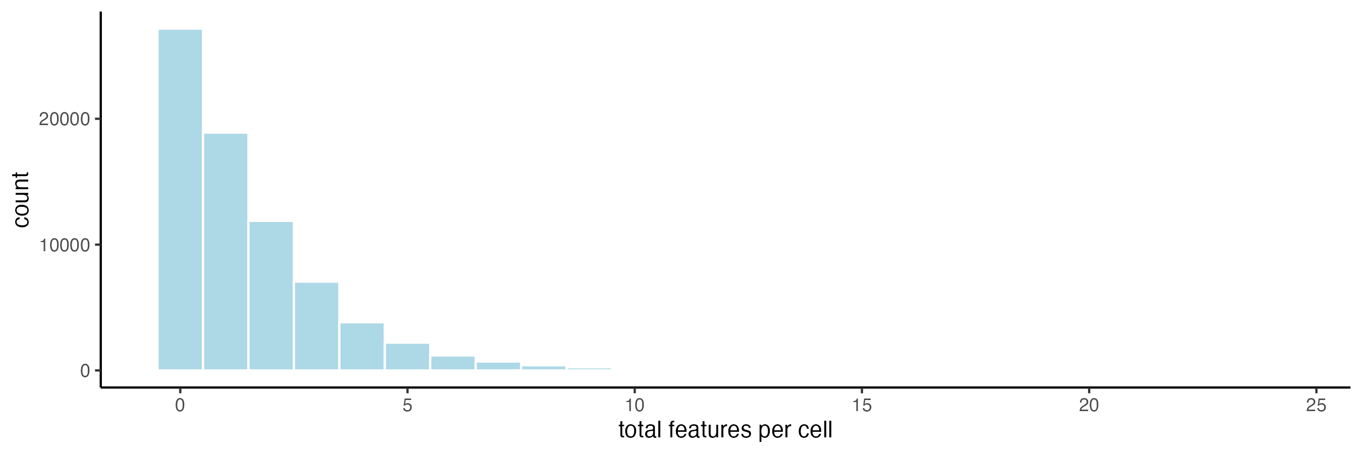
cosmx <- overlapToMatrix(cosmx, feat_info = "negprobes")5.1 Plot histograms of total counts per cell
filterDistributions(cosmx,
    plot_type = "hist",
    detection = "cells",
    method = "sum",
    feat_type = "rna",
    nr_bins = 100,
    save_param = list(
        save_name = "3_filter_dist_rna",
        base_height = 3
    )
)
filterDistributions(cosmx,
    plot_type = "hist",
    detection = "cells",
    method = "sum",
    feat_type = "negprobes",
    nr_bins = 25,
    save_param = list(
        save_name = "4_filter_dist_negprobes",
        base_height = 3
    )
)
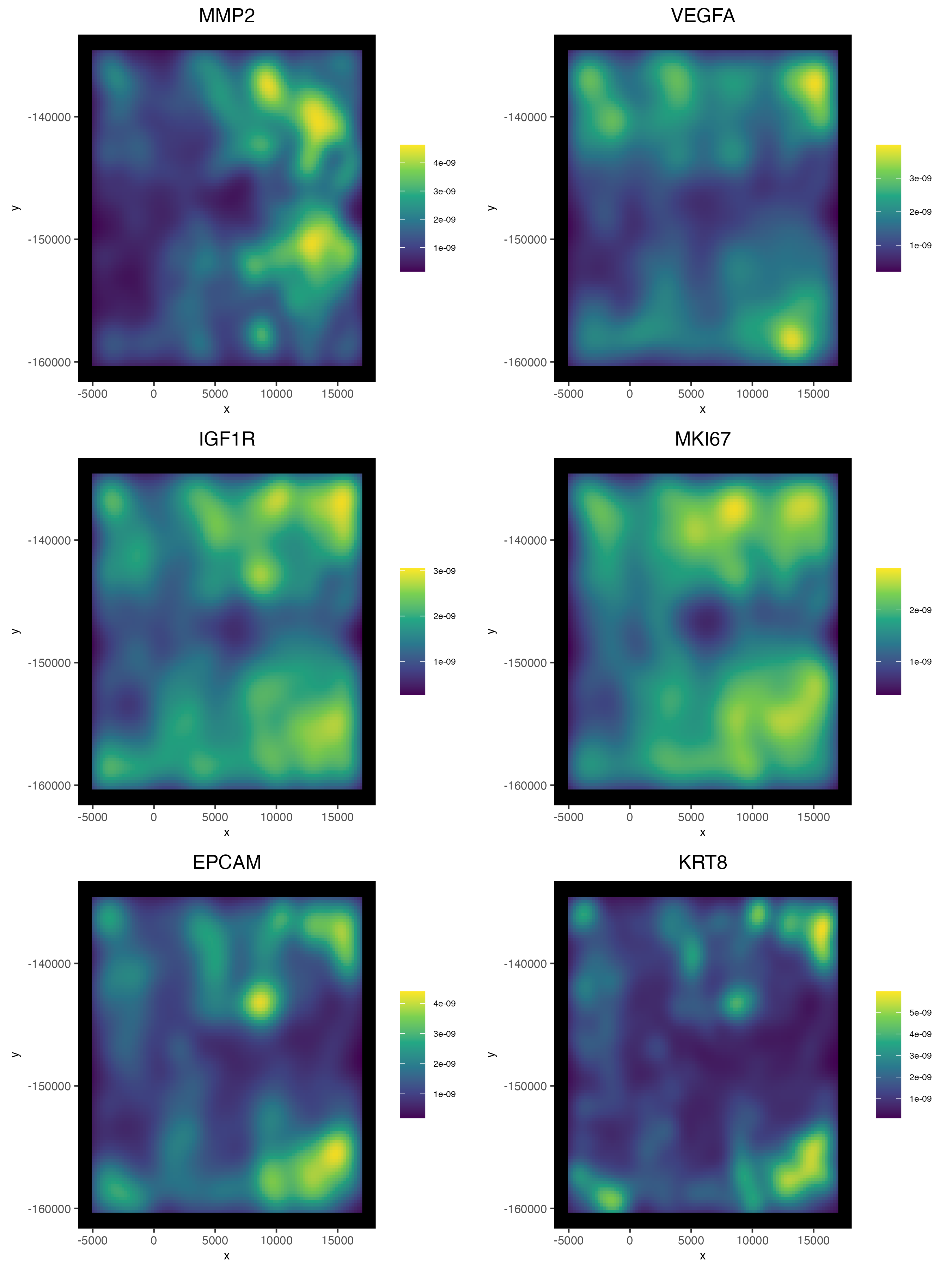
5.2 2D Density Plots
Density-based representations may sometimes be preferred instead of viewing the raw points information, especially when points are dense enough that there is overplotting.
spatInSituPlotDensity(cosmx,
    show_polygon = FALSE,
    use_overlap = FALSE,
    feats = c("MMP2", "VEGFA", "IGF1R",
              "MKI67", "EPCAM", "KRT8"),
    cow_n_col = 2,
    save_param = list(
        base_height = 12,
        base_width = 9,
        save_name = "5_density"
    )
)
6 Filtering and normalization
standard normalization method: library size normalization and log normalization. This method will produce both normalized and scaled values that are be returned as the “normalized” and “scaled”expression matrices respectively. In this tutorial, the normalized values will be used for generating expression statistics and plotting expression values. The scaled values will be ignored. We will also generate normalized values for the negative probes for visualization purposes during which the library normalization step will be skipped.
pearson residuals: A normalization that uses the method described in Lause/Kobak et al, 2021. This produces a set of values that are most similar in utility to a scaled matrix and offer improvements to both HVF detection and PCA generation. These values should not be used for statistics, plotting of expression values, or differential expression analysis.
cosmx <- filterGiotto(cosmx,
    feat_type = "rna",
    expression_threshold = 1,
    feat_det_in_min_cells = 5,
    min_det_feats_per_cell = 5
)

# normalize
# standard method of normalization (log normalization based)
cosmx <- normalizeGiotto(cosmx,
    feat_type = "rna",
    norm_methods = "standard"
)

# new normalization method based on pearson correlations (Lause/Kobak et al. 2021)
# this normalized matrix is given the name "pearson" using the update_slot param
cosmx <- normalizeGiotto(cosmx,
    feat_type = "rna",
    scalefactor = 5000,
    norm_methods = "pearson_resid",
    name = "pearson"
)
# add statistics based on log normalized values
cosmx <- addStatistics(cosmx,
    expression_values = "normalized",
    feat_type = "rna"
)

# add statistics for the raw negative probe values
cosmx <- addStatistics(cosmx,
    expression_values = "raw",
    feat_type = "negprobes"
)

# View cellular data (default is feat = "rna")
showGiottoCellMetadata(cosmx)

# View feature data
showGiottoFeatMetadata(cosmx)
Note: The show functions for metadata do not return
the information. To retrieve the metadata information, instead use
pDataDT() and fDataDT() along with the
feat_type param for either “rna” or “negprobes”.
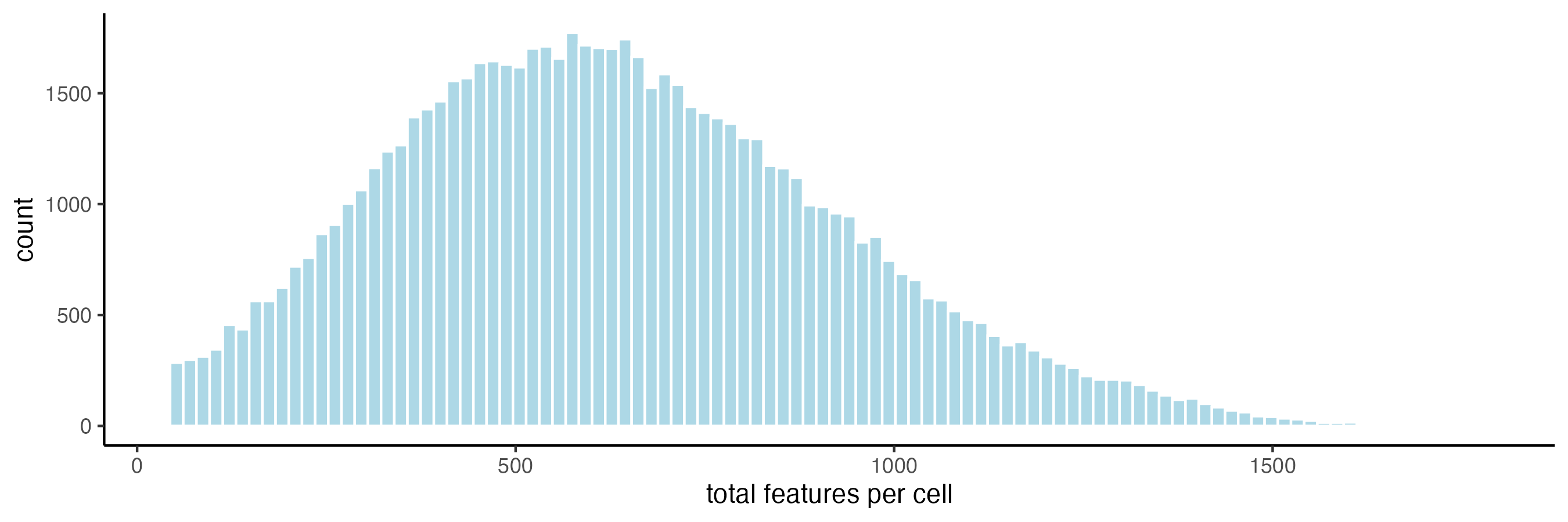
7 View Transcript Total Expression Distribution
7.1 Histogram of log normalized data
filterDistributions(cosmx,
    detection = "cells",
    feat_type = "rna",
    expression_values = "normalized",
    method = "sum",
    nr_bins = 100,
    save_param = list(
        base_height = 3,
        save_name = "6_filter_dist_rna_lognorm"
    )
)
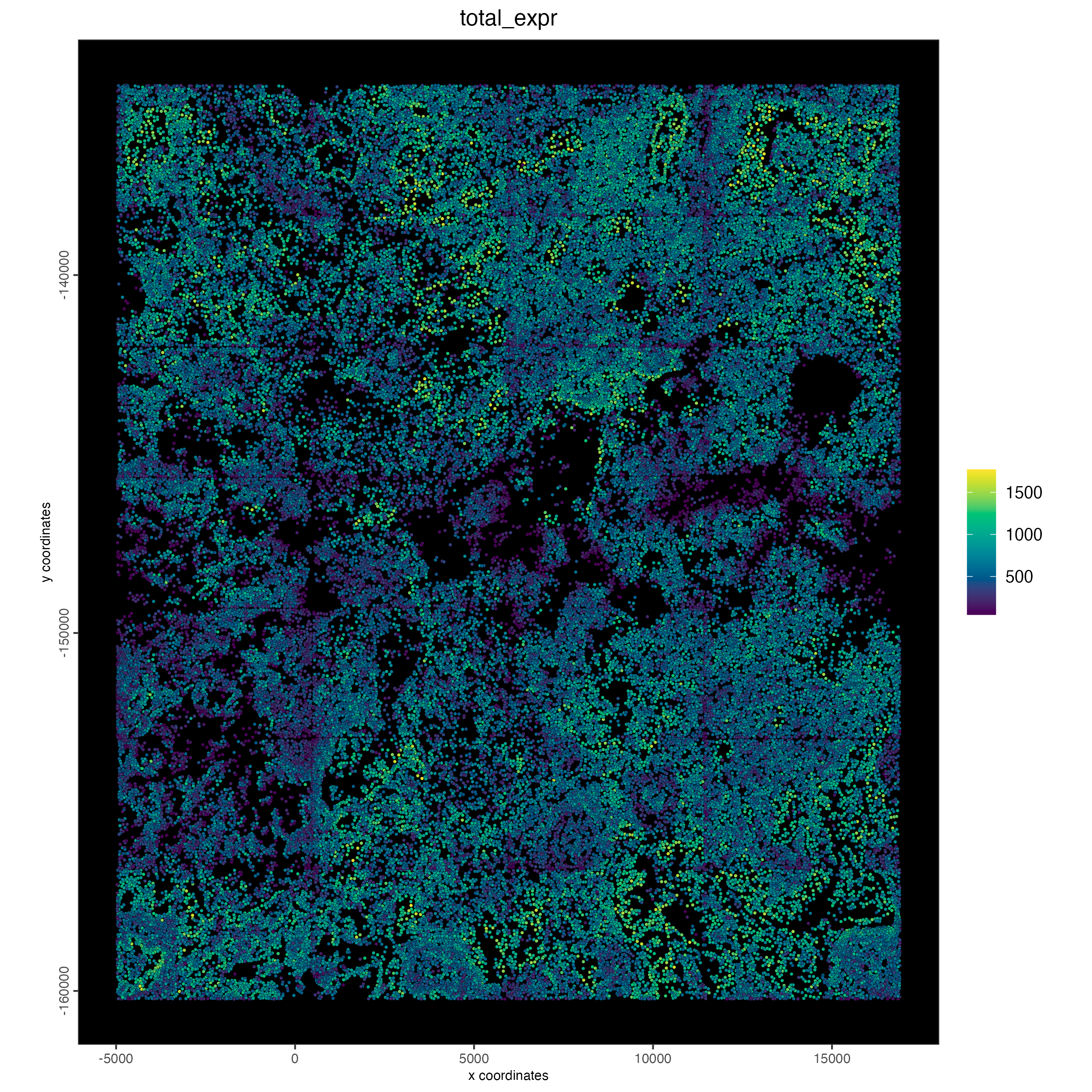
7.2 Plot normalized total expression
spatPlot2D(cosmx,
    cell_color = "total_expr",
    gradient_style = "sequential",
    color_as_factor = FALSE,
    point_size = 0.9,
    background_color = "black",
    save_param = list(
        save_name = "8_normexp"
    )
)
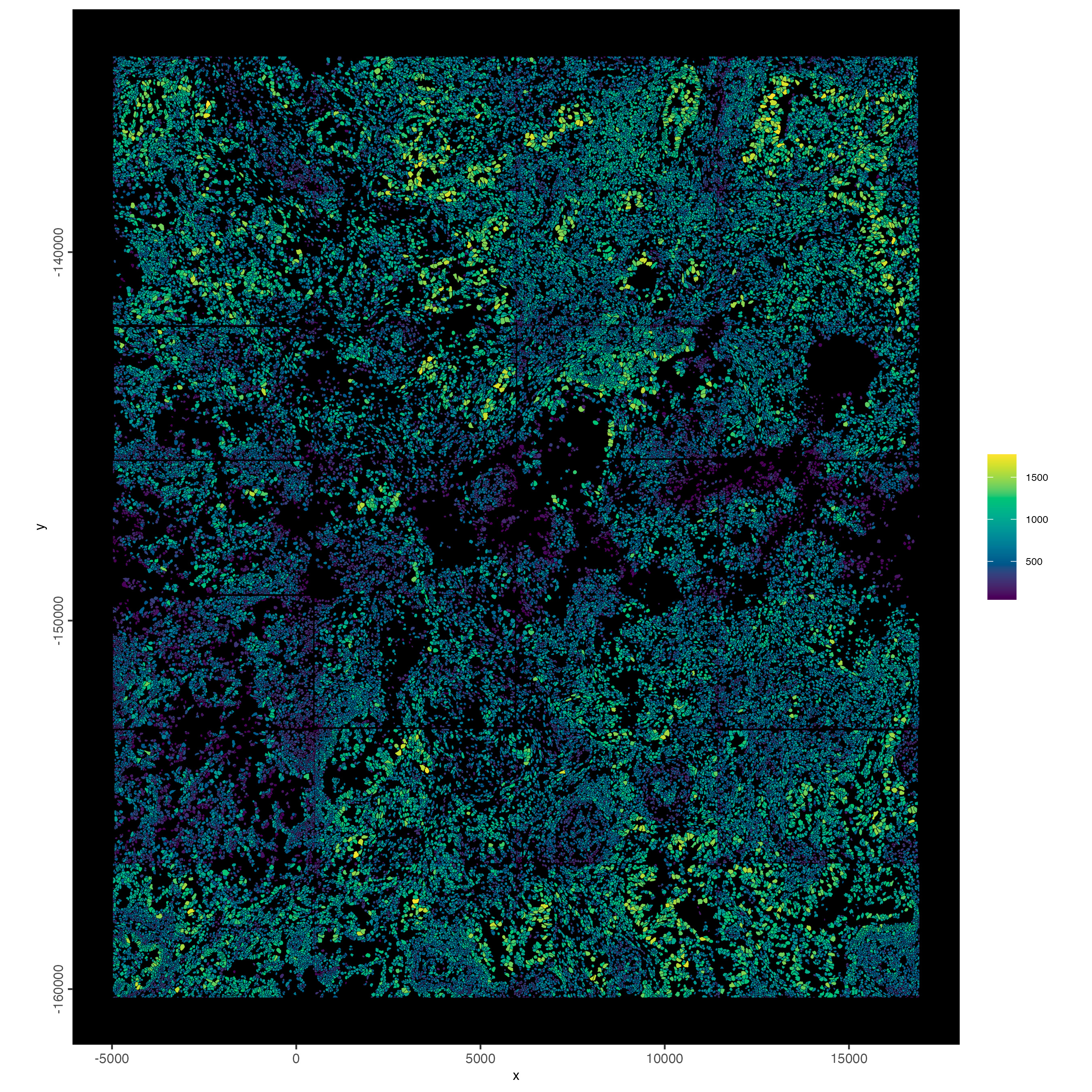
7.3 Plot spatially as color-scaled polygons
spatInSituPlotPoints(cosmx,
    show_polygon = TRUE,
    polygon_fill_gradient_style = "sequential",
    polygon_color = "black",
    polygon_line_size = 0.05,
    polygon_fill = "total_expr",
    polygon_fill_as_factor = FALSE,
    save_param = list(
        save_name = "9_total_expr"
    )
)
8 Dimension Reduction
8.1 Detect highly variable genes and generate PCA
Detect highly variable genes using the pearson residuals method based on the “pearson” expression matrix. These results will be returned as a new “hvf” column in the “rna” feature metadata.
PCA generation will also be based on the “pearson” matrix. Scaling and centering of the PCA which is usually done by default will be skipped since the pearson matrix is already scaled.
cosmx <- calculateHVF(cosmx,
    method = "var_p_resid",
    var_number = 500, # leaving as NULL results in too few genes to use
    save_plot = TRUE,
    save_param = list(
        save_name = "10_hvf"
    )
)
# If you get an Error related to future.apply, please modify the maximum size
# of global variables by running: options(future.globals.maxSize = 1e10)

# print HVFs
gene_metadata <- fDataDT(cosmx)
gene_metadata[hvf == "yes", feat_ID]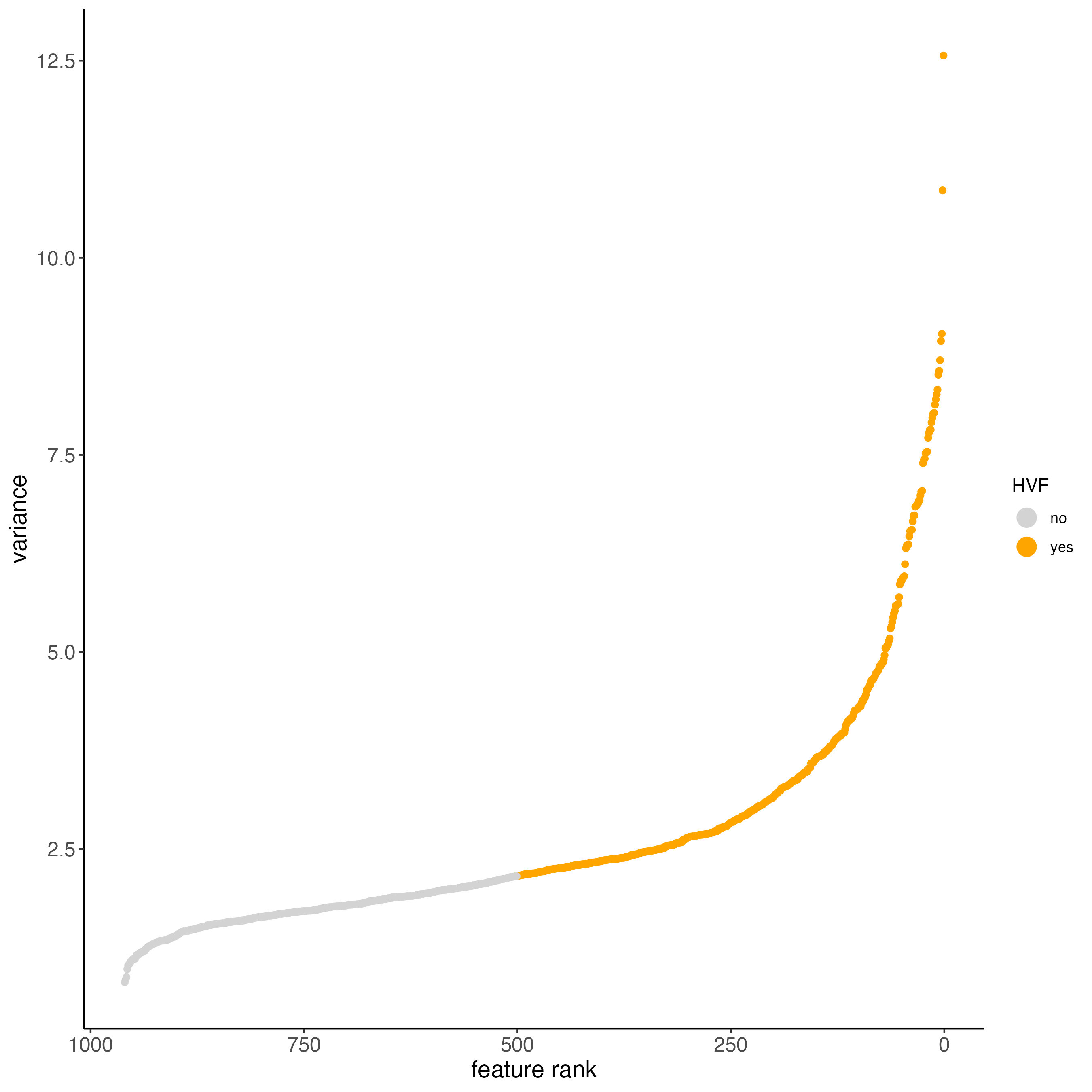
cosmx <- runPCA(cosmx,
scale_unit = FALSE,
center = FALSE,
expression_values = "pearson"
)
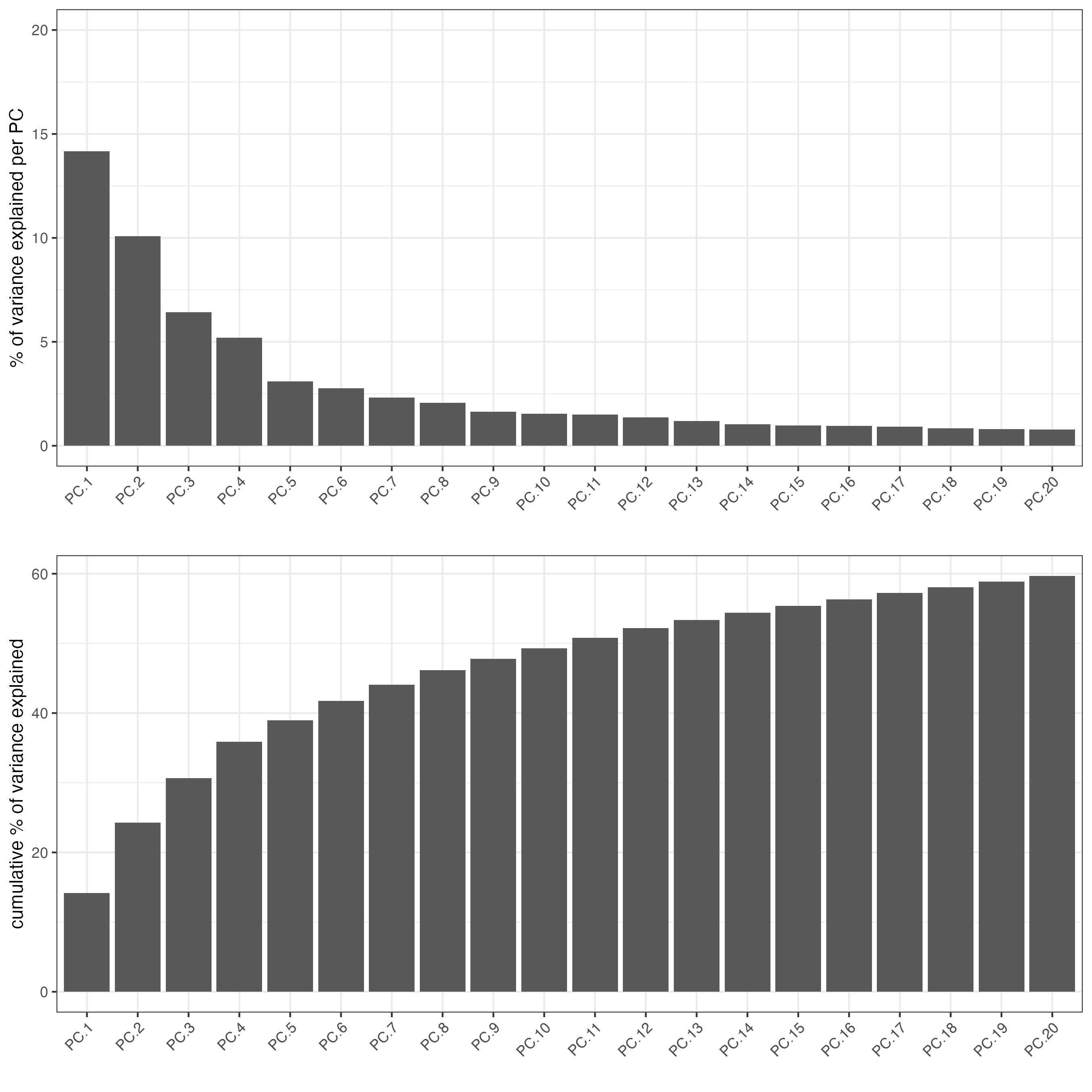
# screeplot uses the generated PCA. No need to specify expr values
screePlot(cosmx,
ncp = 20,
save_param = list(
save_name = "11_scree"
)
)
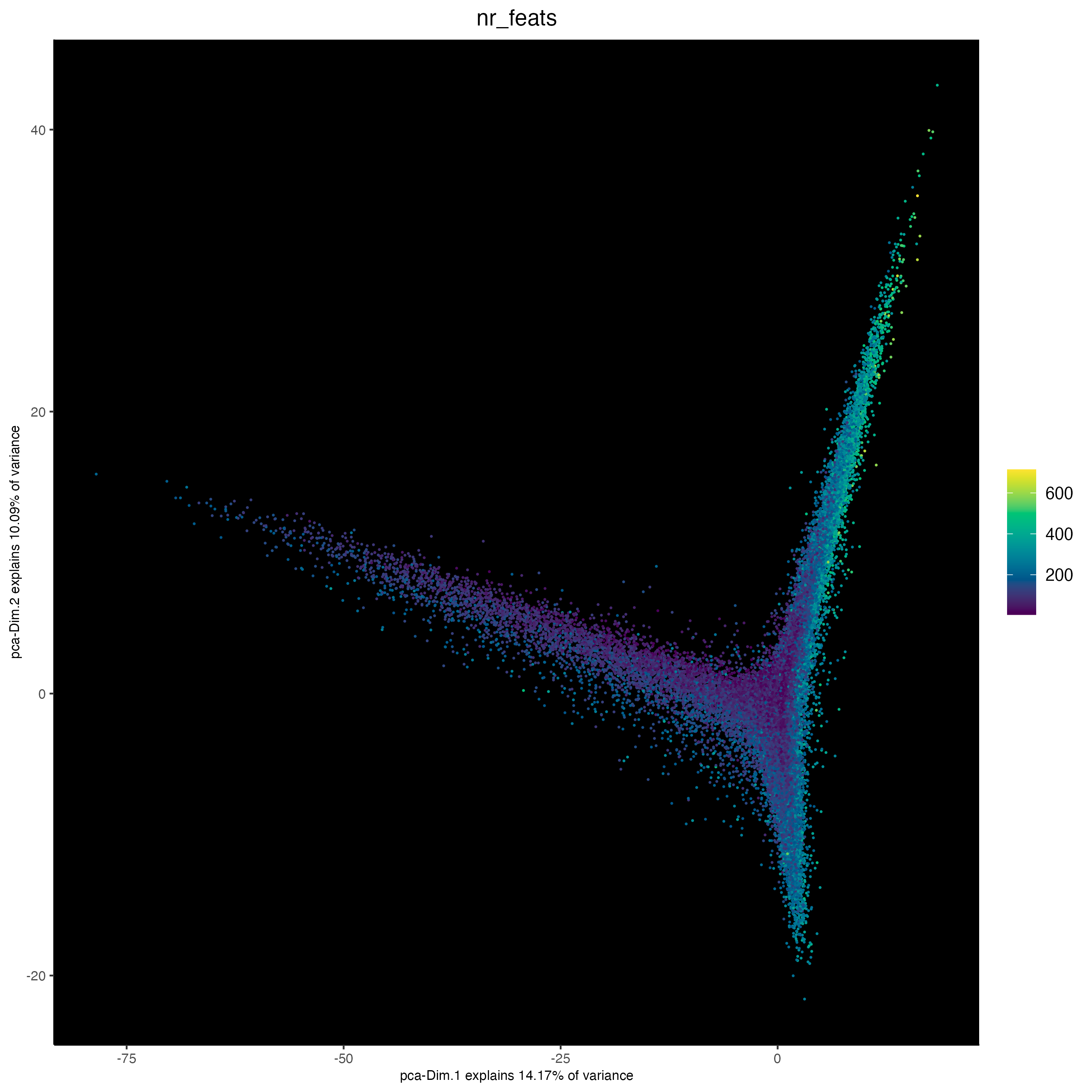
plotPCA(cosmx,
    cell_color = "nr_feats", # (from log normed expression statistics)
    color_as_factor = FALSE,
    point_size = 0.8,
    gradient_style = "sequential",
    point_border_stroke = 0,
    background_color = "black",
    save_param = list(
        save_name = "12_pca"
    )
)
8.2 Run tSNE and UMAP
cosmx <- runtSNE(cosmx,
dimensions_to_use = 1:10
)
cosmx <- runUMAP(cosmx,
dimensions_to_use = 1:10
)
plotTSNE(cosmx,
cell_color = "fov",
show_center_label = FALSE,
save_param = list(
save_name = "13_tsne_fov"
)
)
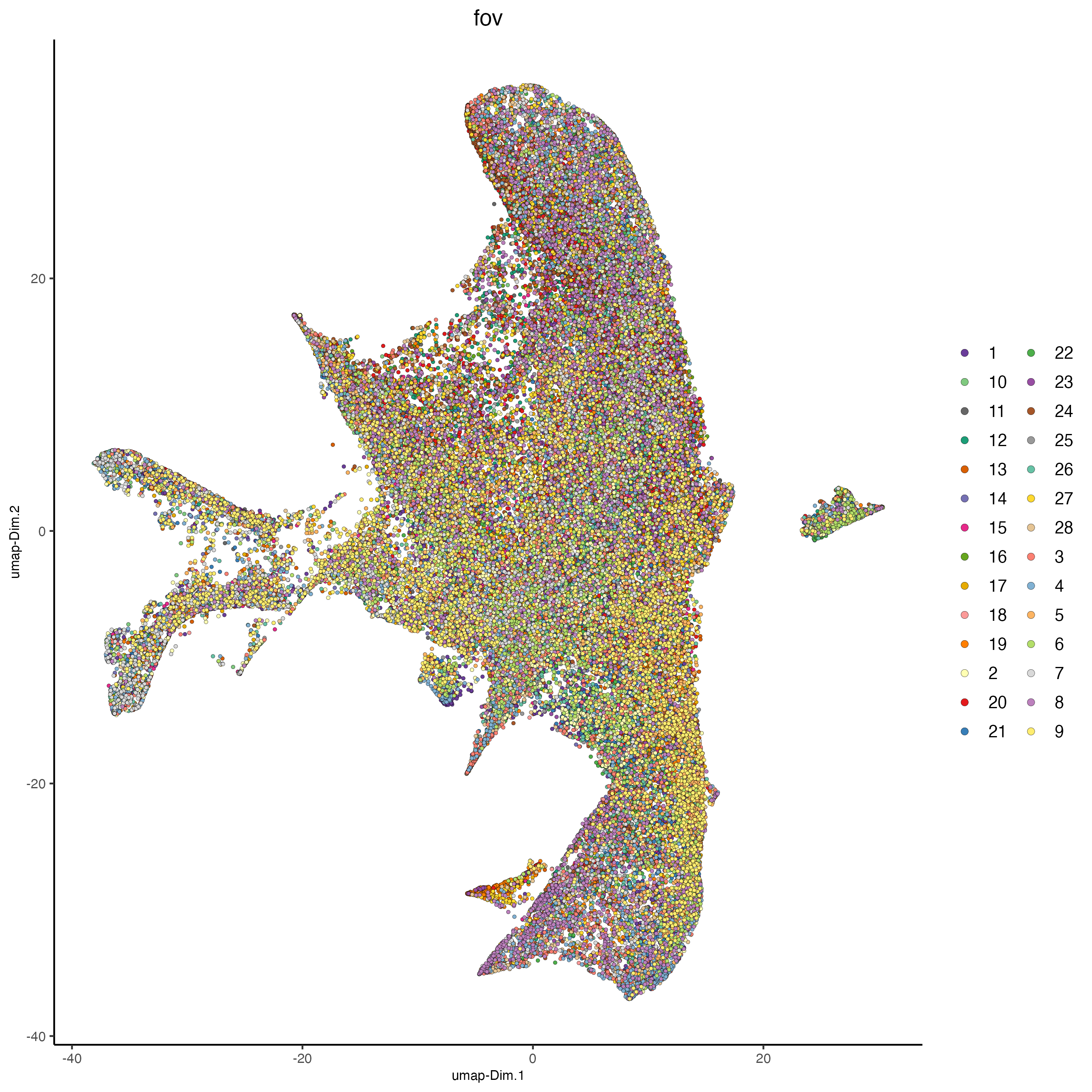
showGiottoDimRed(cosmx)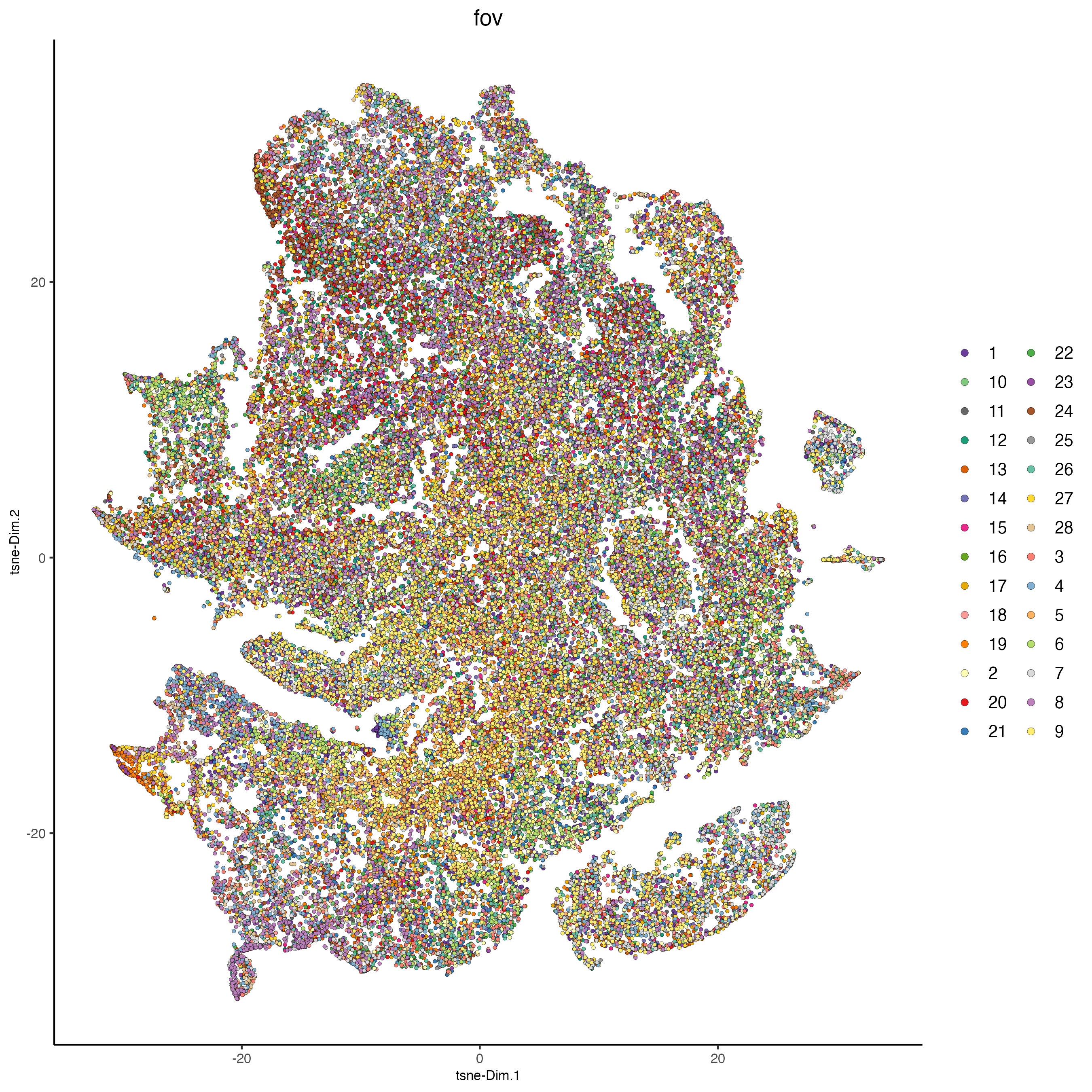
plotUMAP(cosmx,
    cell_color = "fov",
    show_center_label = FALSE,
    save_param = list(
        save_name = "14_umap_fov"
    )
)
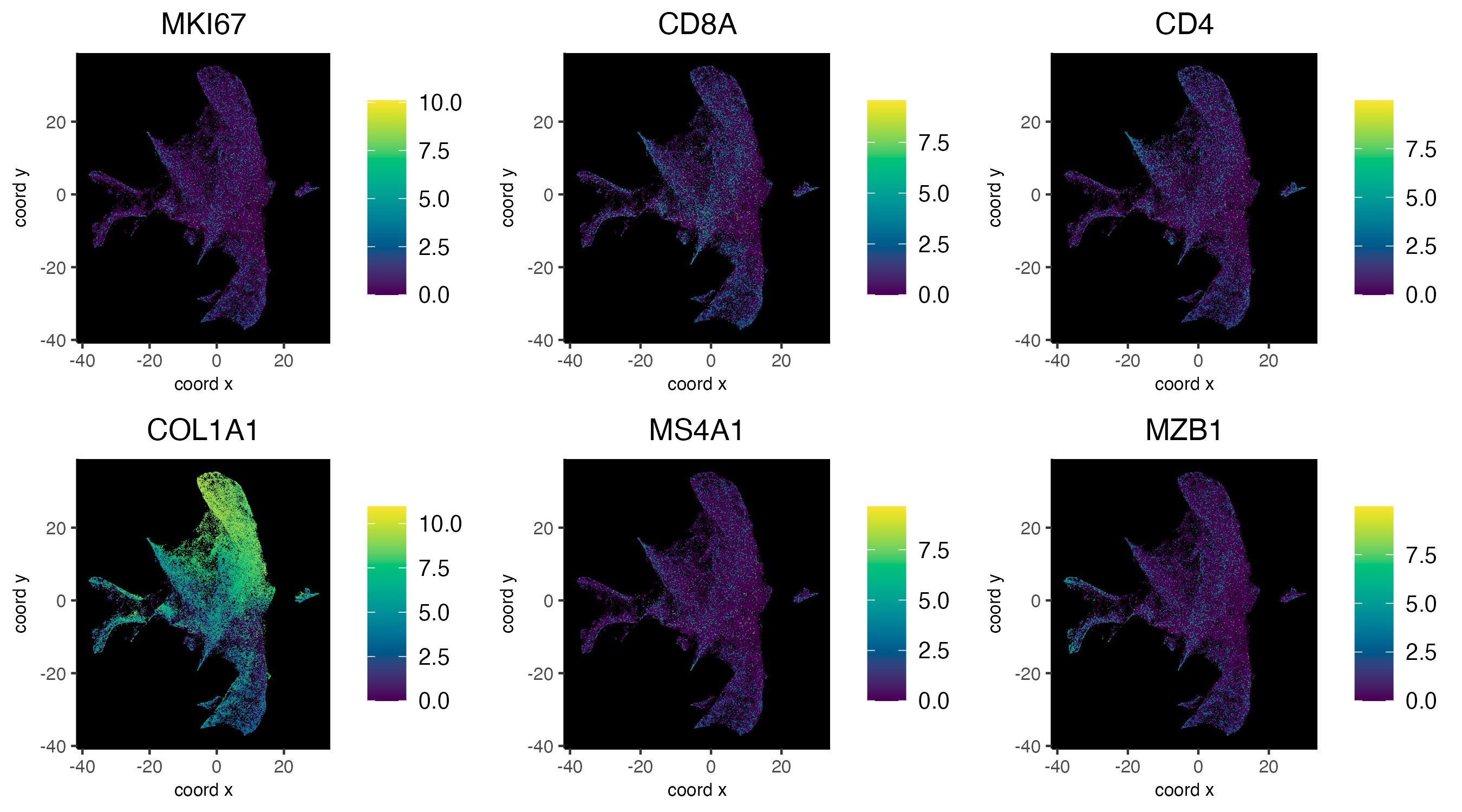
8.3 Plot features on expression space
dimFeatPlot2D(cosmx,
    feats = c(
        "MKI67", "CD8A", "CD4", "COL1A1", "MS4A1", "MZB1"),
    expression_values = "normalized",
    gradient_style = "sequential",
    point_border_stroke = 0,
    point_size = 0.2,
    cow_n_col = 3,
    background_color = "black",
    save_param = list(
        base_height = 5,
        save_name = "15_dfp_umap"
    )
)
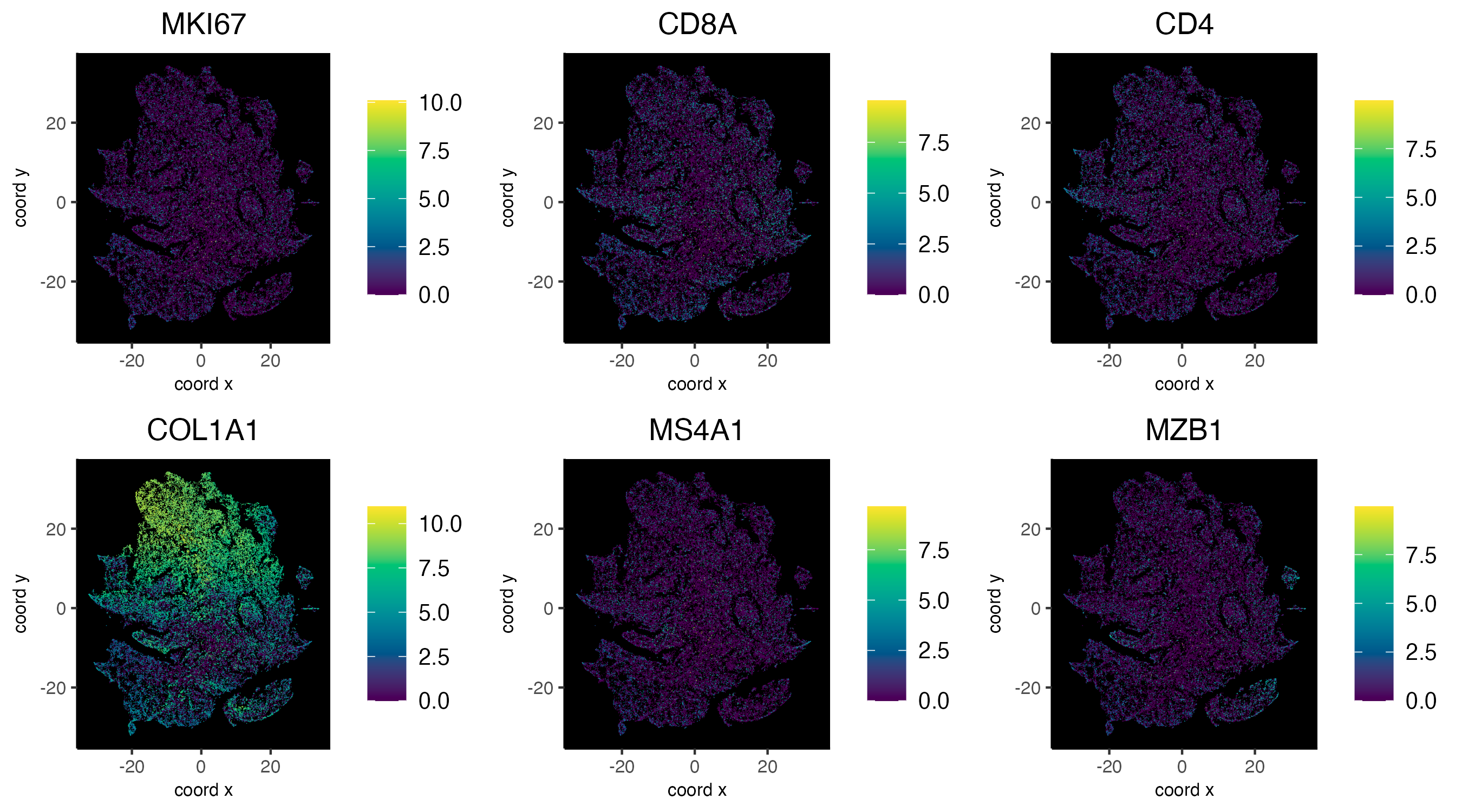
dimFeatPlot2D(cosmx,
    feats = c(
        "MKI67", "CD8A", "CD4", "COL1A1", "MS4A1", "MZB1"),
    expression_values = "normalized",
    dim_reduction_to_use = "tsne",
    dim_reduction_name = "tsne",
    gradient_style = "sequential",
    point_border_stroke = 0,
    point_size = 0.2,
    cow_n_col = 3,
    background_color = "black",
    save_param = list(
        base_height = 5,
        save_name = "16_dfp_tsne"
    )
)
9 Cluster
9.1 Visualize clustering
cosmx <- createNearestNetwork(cosmx,
dimensions_to_use = 1:10,
k = 10
)
cosmx <- doLeidenCluster(cosmx,
resolution = 0.07,
n_iterations = 100
)
clus_colors <- getColors("Vivid", 10)
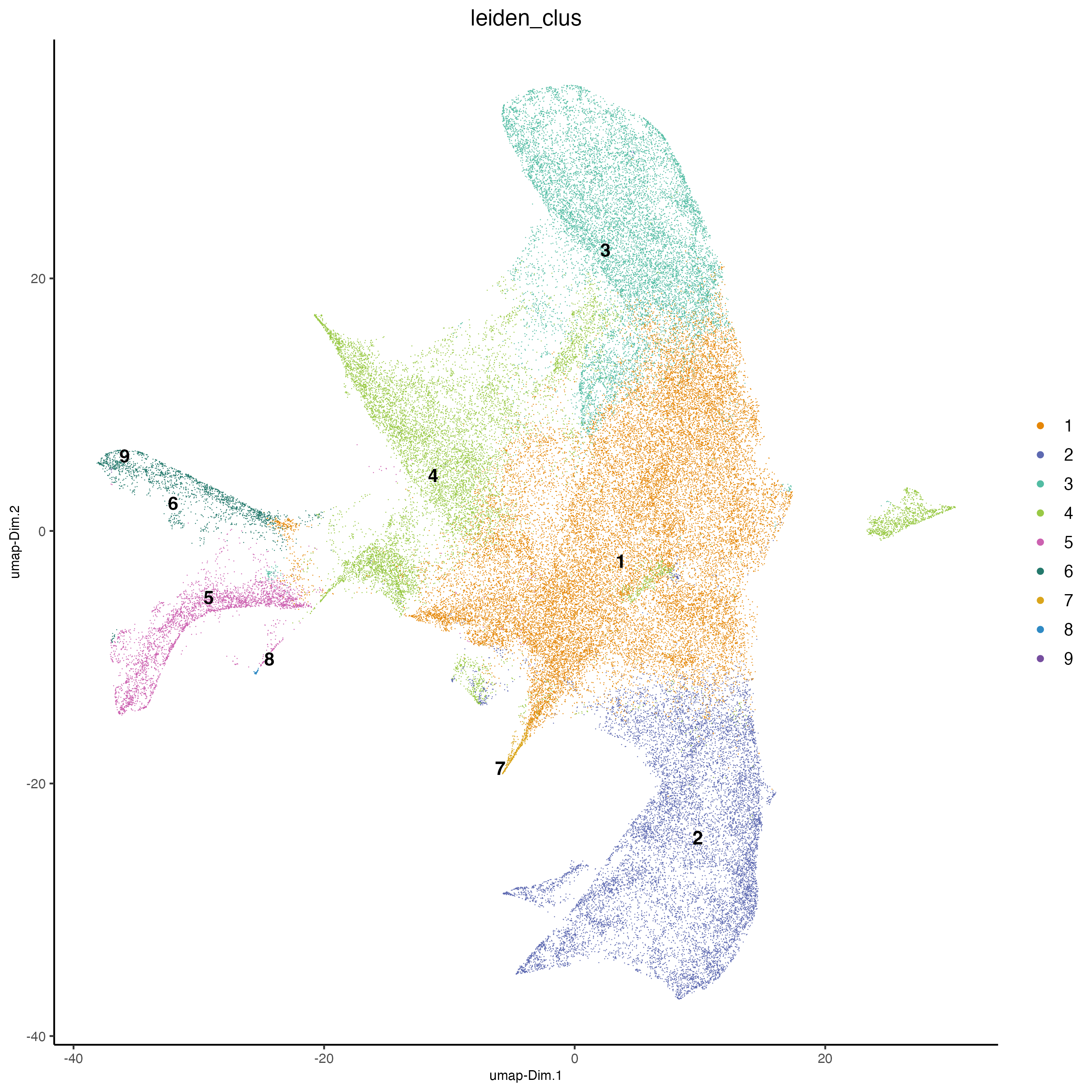
# visualize UMAP cluster results
plotUMAP(cosmx,
cell_color = "leiden_clus",
cell_color_code = clus_colors,
point_border_stroke = 0,
point_size = 0.3,
save_param = list(
save_name = "17_leiden_umap"
)
)
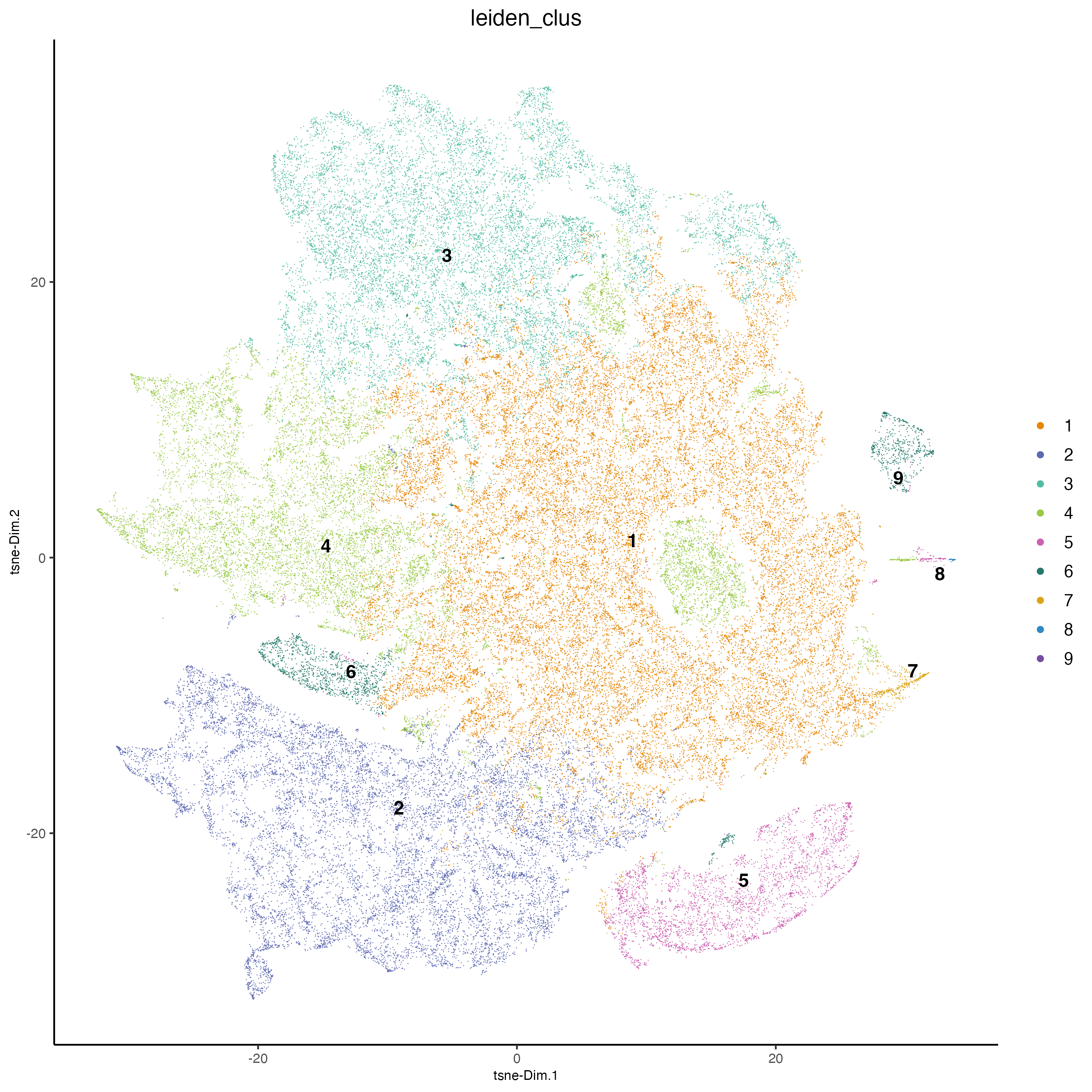
plotTSNE(cosmx,
    cell_color = "leiden_clus",
    cell_color_code = clus_colors,
    point_border_stroke = 0,
    point_size = 0.3,
    save_param = list(
        save_name = "18_leiden_tsne"
    )
)
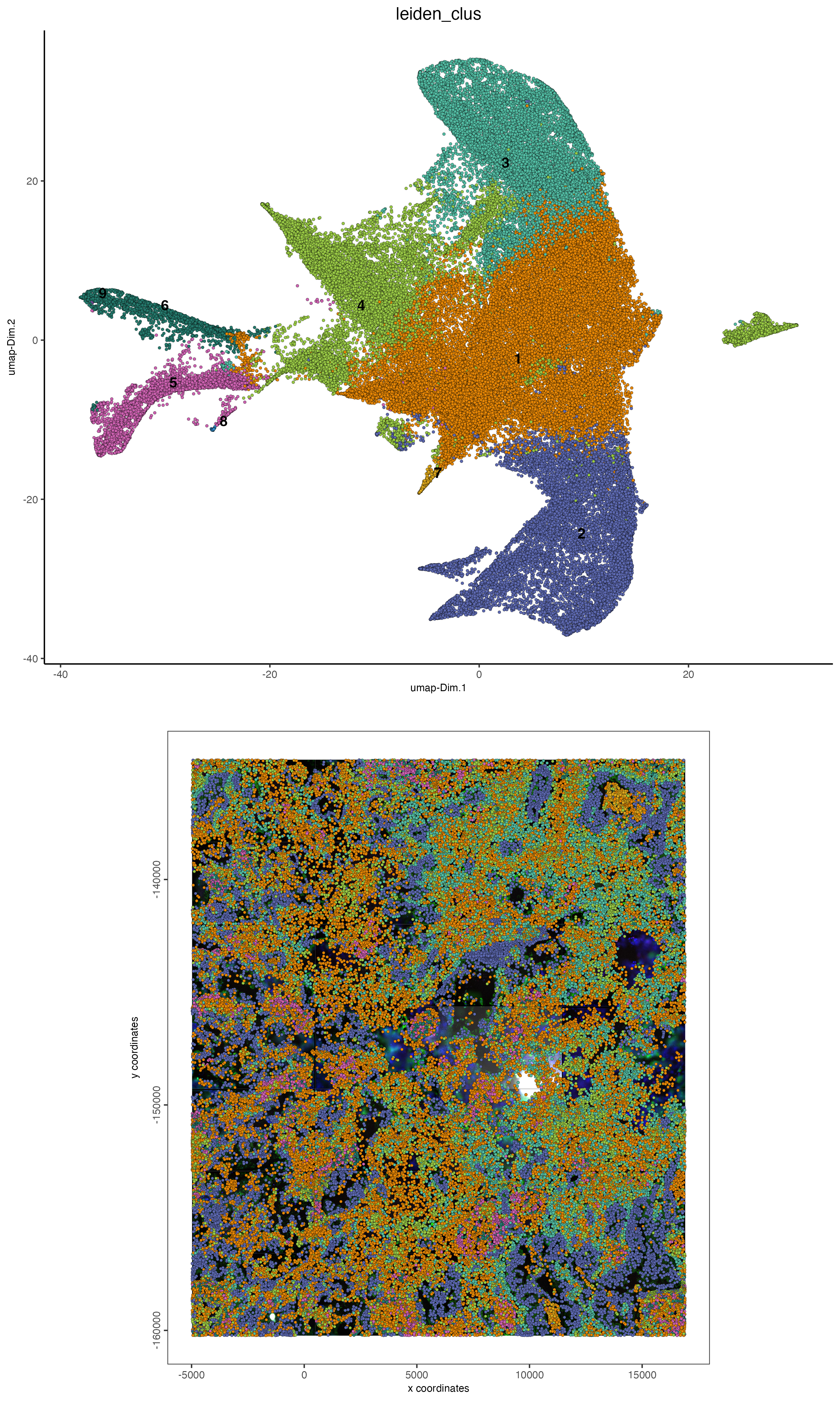
9.2 Visualize clustering on expression and spatial space
# visualize UMAP and spatial results
spatDimPlot2D(cosmx,
    show_image = TRUE,
    image_name = image_names,
    cell_color = "leiden_clus",
    cell_color_code = clus_colors,
    spat_point_size = 1,
    save_param = list(
        base_width = 9,
        base_height = 15,
        save_name = "19_sdplot"
    )
)
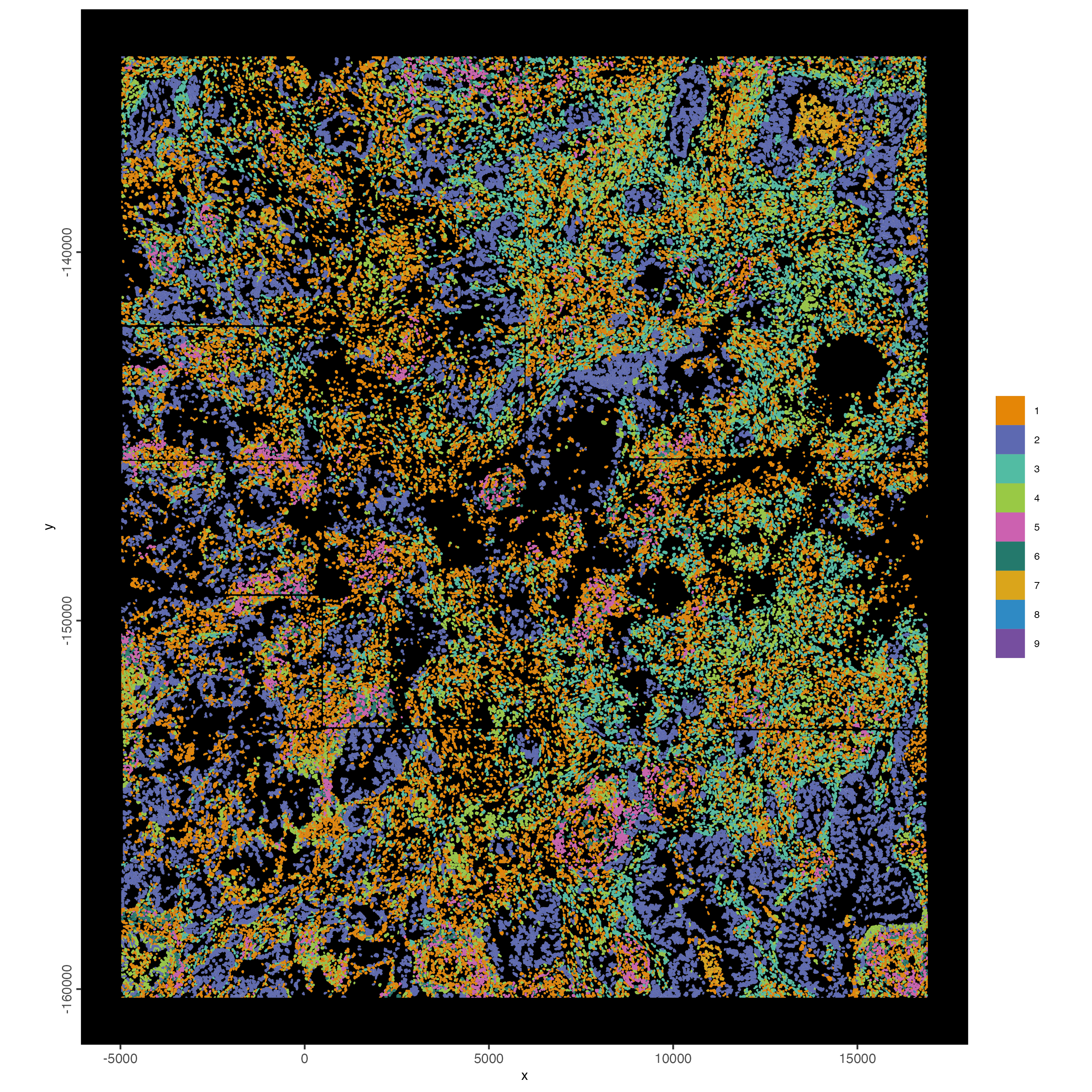
9.3 Map clustering spatially
spatInSituPlotPoints(cosmx,
    show_polygon = TRUE,
    polygon_color = "white",
    polygon_line_size = 0.01,
    polygon_fill = "leiden_clus",
    polygon_fill_as_factor = TRUE,
    polygon_fill_code = clus_colors,
    save_param = list(
        save_name = "20_sisp_leiden"
    )
)
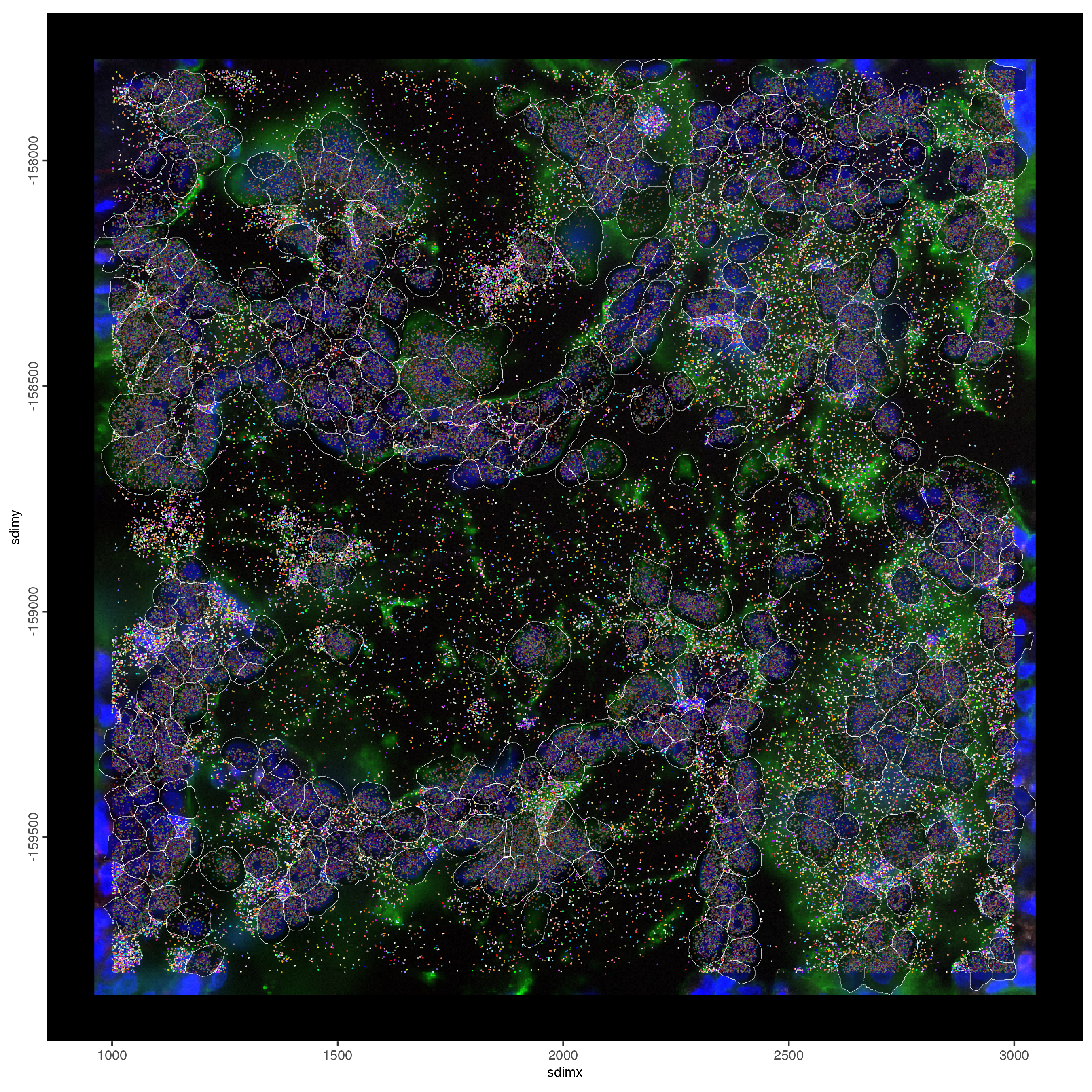
10 Small Subset Visualization
#subset a Giotto object based on spatial locations
smallfov <- subsetGiottoLocs(cosmx,
    x_max = 3000,
    x_min = 1000,
    y_max = -157800,
    y_min = -159800
)

#extract all genes observed in new object
smallfeats <- fDataDT(smallfov)[, feat_ID]

#plot all genes
spatInSituPlotPoints(smallfov,
    feats = list(smallfeats),
    point_size = 0.15,
    polygon_line_size = 0.1,
    show_polygon = TRUE,
    use_overlap = FALSE,
    polygon_color = "white",
    show_image = TRUE,
    image_name = "composite_fov002",
    show_legend = FALSE,
    save_param = list(
        save_name = "21_smallfov1"
    )
)
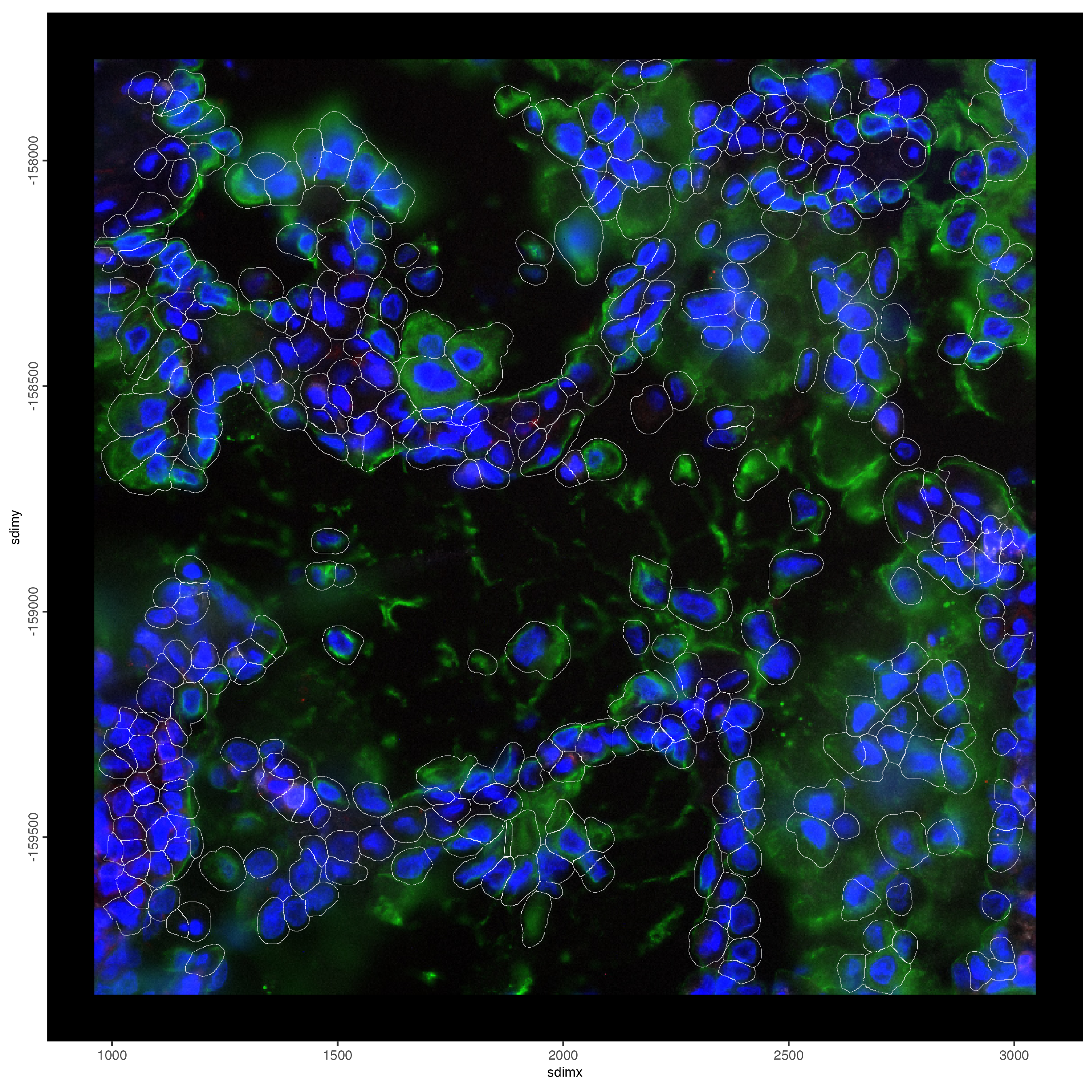
# plot only the polygon outlines
spatInSituPlotPoints(smallfov,
    polygon_line_size = 0.1,
    polygon_alpha = 0,
    polygon_color = "white",
    show_polygon = TRUE,
    show_image = TRUE,
    image_name = "composite_fov002",
    show_legend = FALSE,
    save_param = list(
        save_name = "22_smallfov2"
    )
)
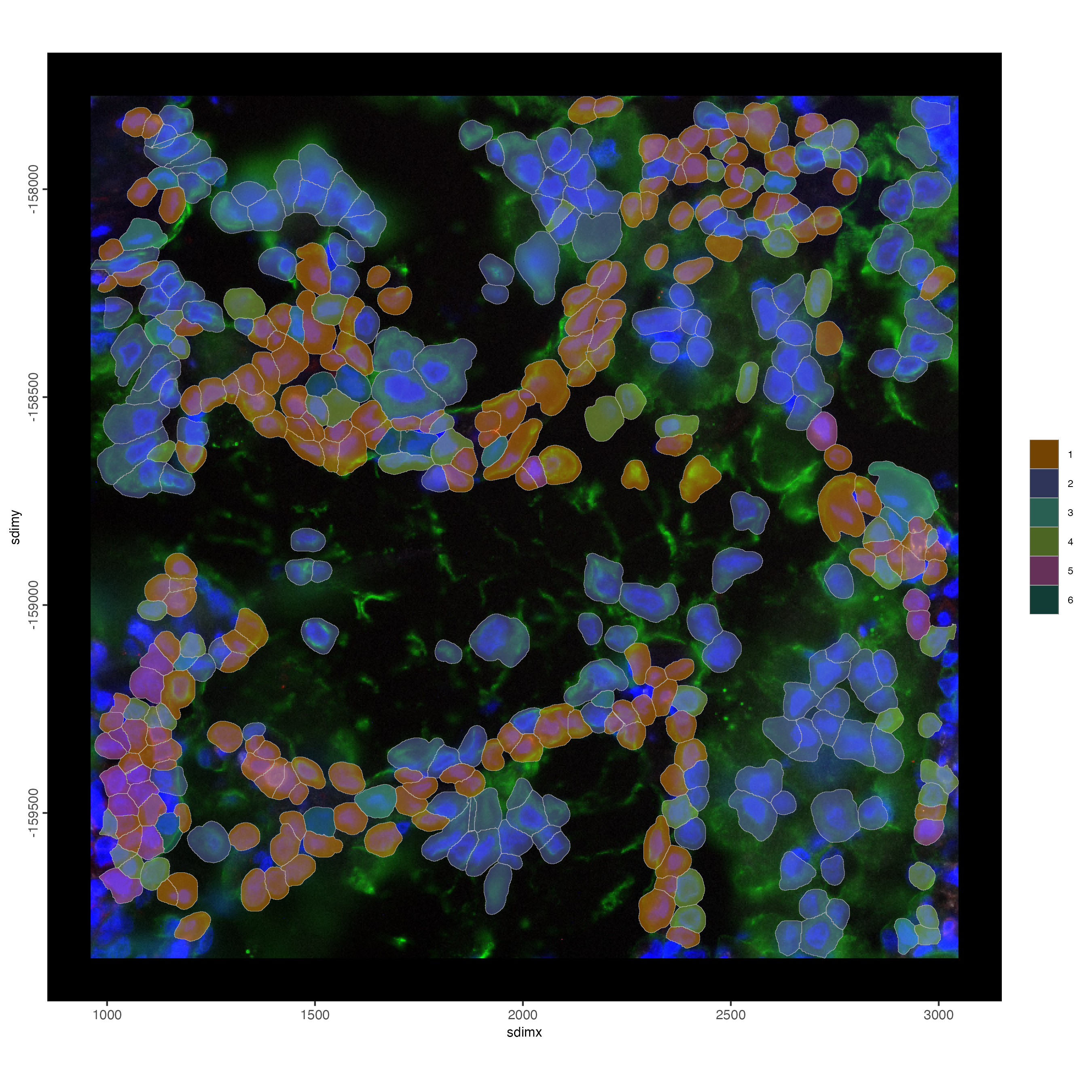
# plot polygons colorlabeled with leiden clusters
spatInSituPlotPoints(smallfov,
    polygon_line_size = 0.1,
    show_polygon = TRUE,
    polygon_fill = "leiden_clus",
    polygon_fill_as_factor = TRUE,
    polygon_fill_code = clus_colors,
    show_image = TRUE,
    image_name = "composite_fov002",
    show_legend = FALSE,
    save_param = list(
        save_name = "23_smallfov3"
    )
)
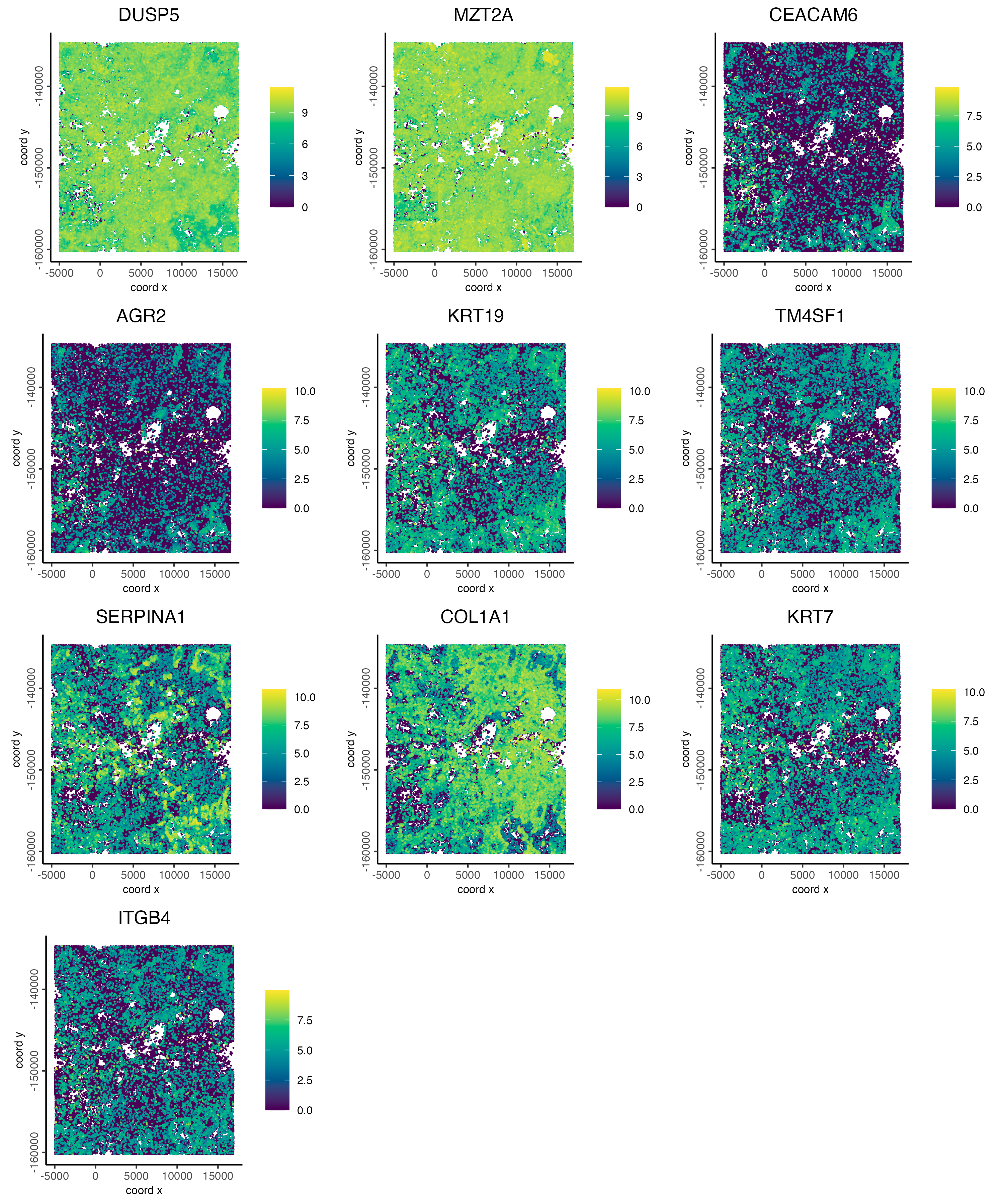
11 Spatial Expression Patterns
Find spatially organized gene expression by examining the binarized expression of cells and their spatial neighbors.
# create spatial network based on physical distance of cell centroids
cosmx <- createSpatialNetwork(cosmx,
    minimum_k = 2,
    maximum_distance_delaunay = 50
)

# perform Binary Spatial Extraction of genes - NOTE: Depending on your system this could take time
km_spatialfeats <- binSpect(cosmx)

# visualize spatial expression of selected genes obtained from binSpect
spatFeatPlot2D(cosmx,
    expression_values = "normalized",
    feats = km_spatialfeats$feats[1:10],
    point_shape = "no_border",
    point_border_stroke = 0.01,
    point_size = 0.01,
    cow_n_col = 3,
    gradient_style = "sequential",
    save_param = list(
        base_height = 12,
        base_width = 10,
        save_name = "24_top_binspect_spat"
    )
)
12 Identify cluster differential expression genes
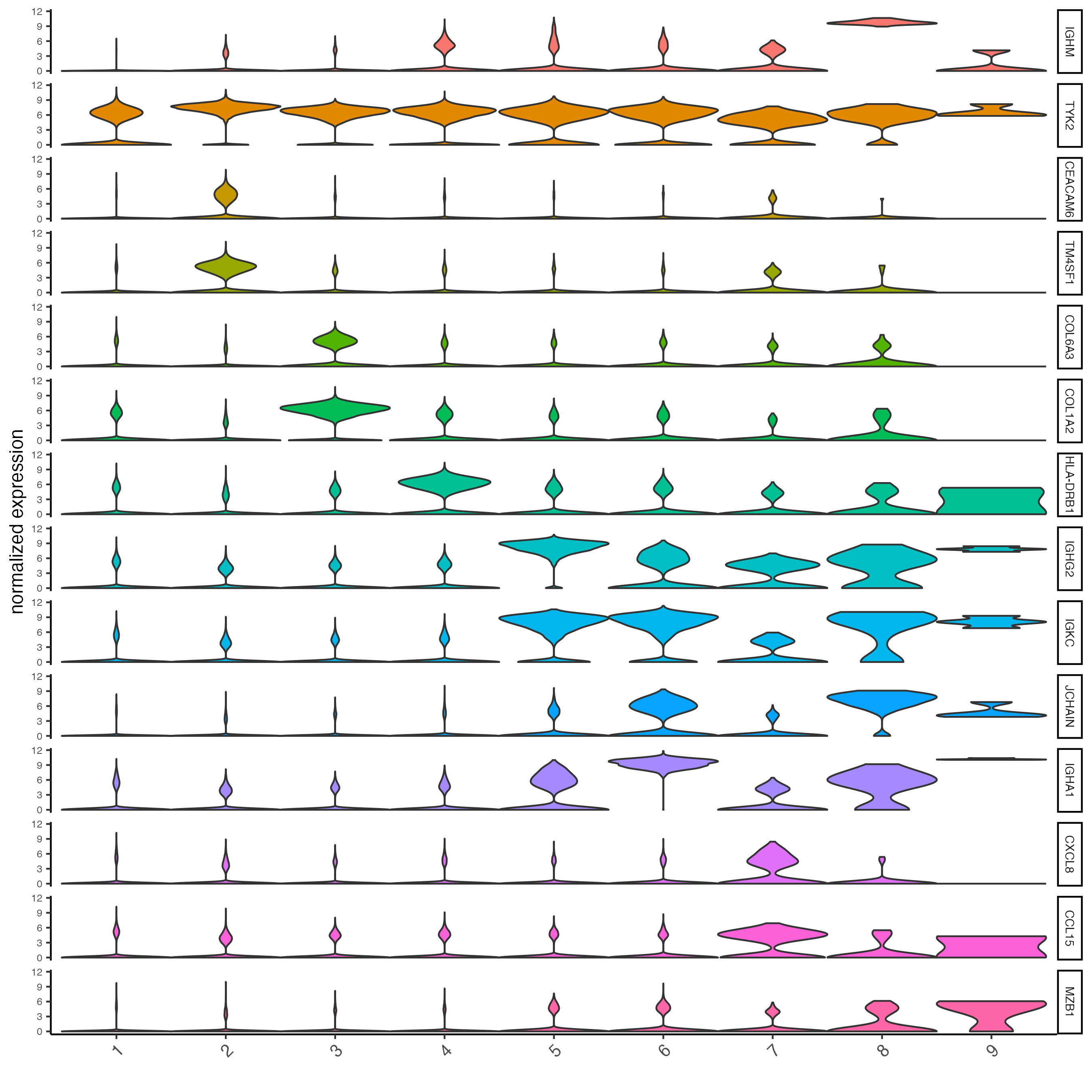
12.1 Violin plot
# Gini
markers_gini <- findMarkers_one_vs_all(cosmx,
    method = "gini",
    expression_values = "normalized",
    cluster_column = "leiden_clus",
    min_feats = 1,
    rank_score = 2
)

# First 5 results by cluster
markers_gini[, head(.SD, 5), by = "cluster"]

# violinplot
topgenes_gini <- unique(markers_gini[, head(.SD, 2), by = "cluster"]$feats)

violinPlot(cosmx,
    feats = topgenes_gini,
    cluster_column = "leiden_clus",
    strip_position = "right",
    save_param = list(
        save_name = "25_vplot"
    )
)
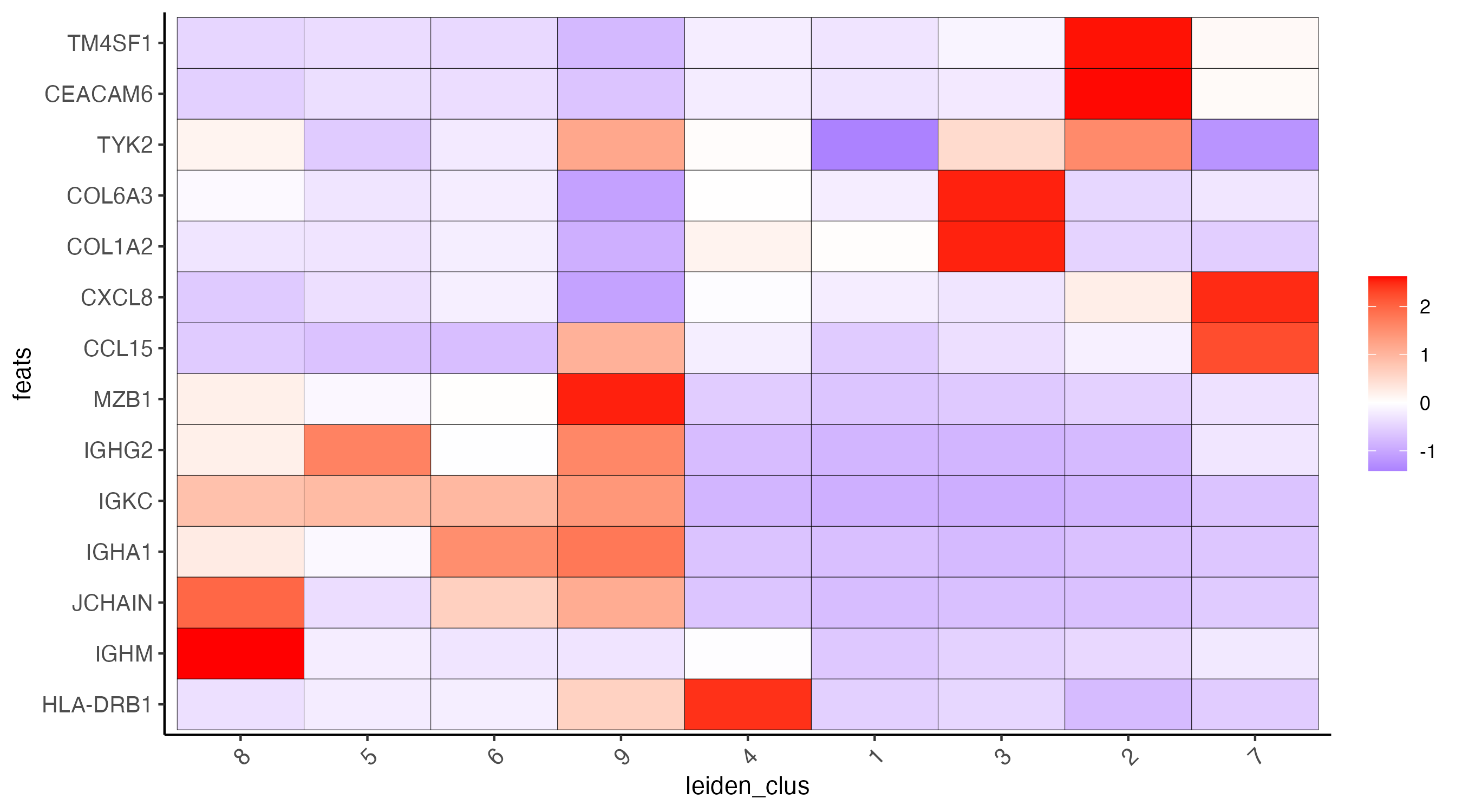
12.2 Heatmap
plotMetaDataHeatmap(cosmx,
    expression_values = "normalized",
    metadata_cols = "leiden_clus",
    selected_feats = topgenes_gini,
    save_param = list(
        base_height = 5,
        save_name = "26_heatmap_gini"
    )
)
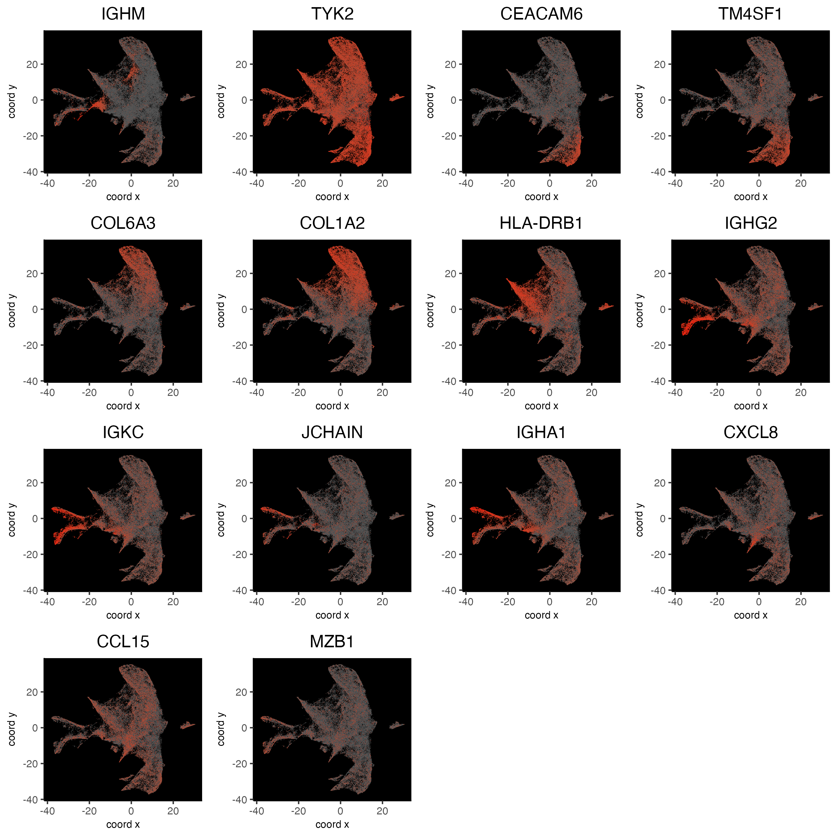
12.3 Plot gini genes on UMAP
# low, mid, high
custom_scale = c("#555555", "red")

dimFeatPlot2D(cosmx,
    cell_color_gradient = custom_scale,
    feats = topgenes_gini,
    point_border_stroke = 0,
    point_size = 0.2,
    cow_n_col = 4,
    show_legend = FALSE,
    background_color = "black",
    save_param = list(
        save_name = "27_dfp_gini"
    )
)
12.4 Protein staining info
spatPlot2D(cosmx,
    cell_color = "Mean.CD3",
    gradient_style = "sequential",
    gradient_limits = c(0, 300), # custom setting so we can see the non-artefacted values
    color_as_factor = FALSE,
    point_border_stroke = 0,
    point_size = 0.8,
    background_color = "black",
    save_param = list(
        save_name = "28_spat_cd3"
    )
)
# fovs 11,12,14,15,16 are artefacted for CD3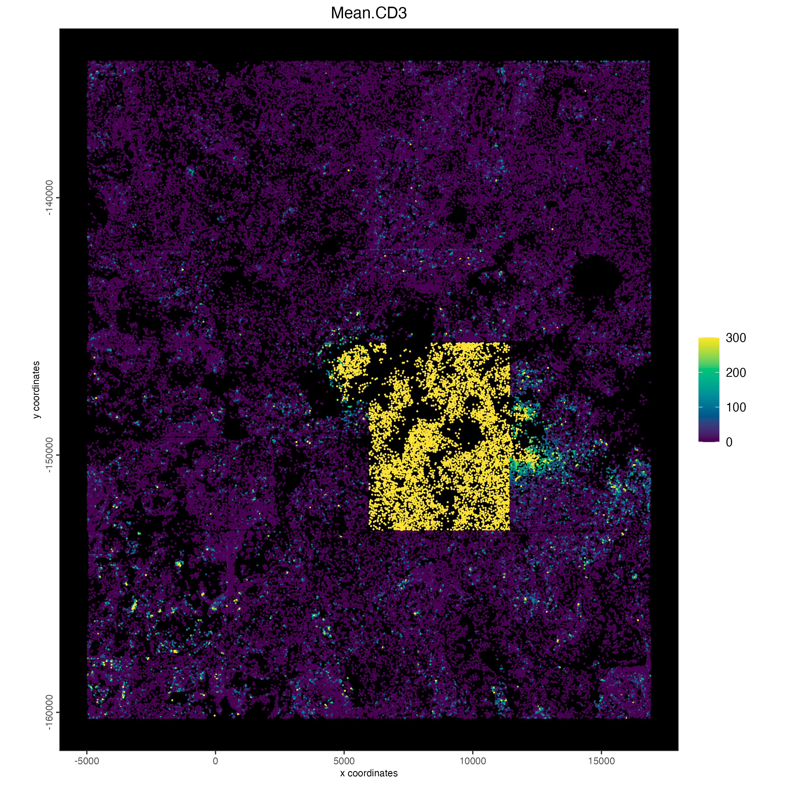
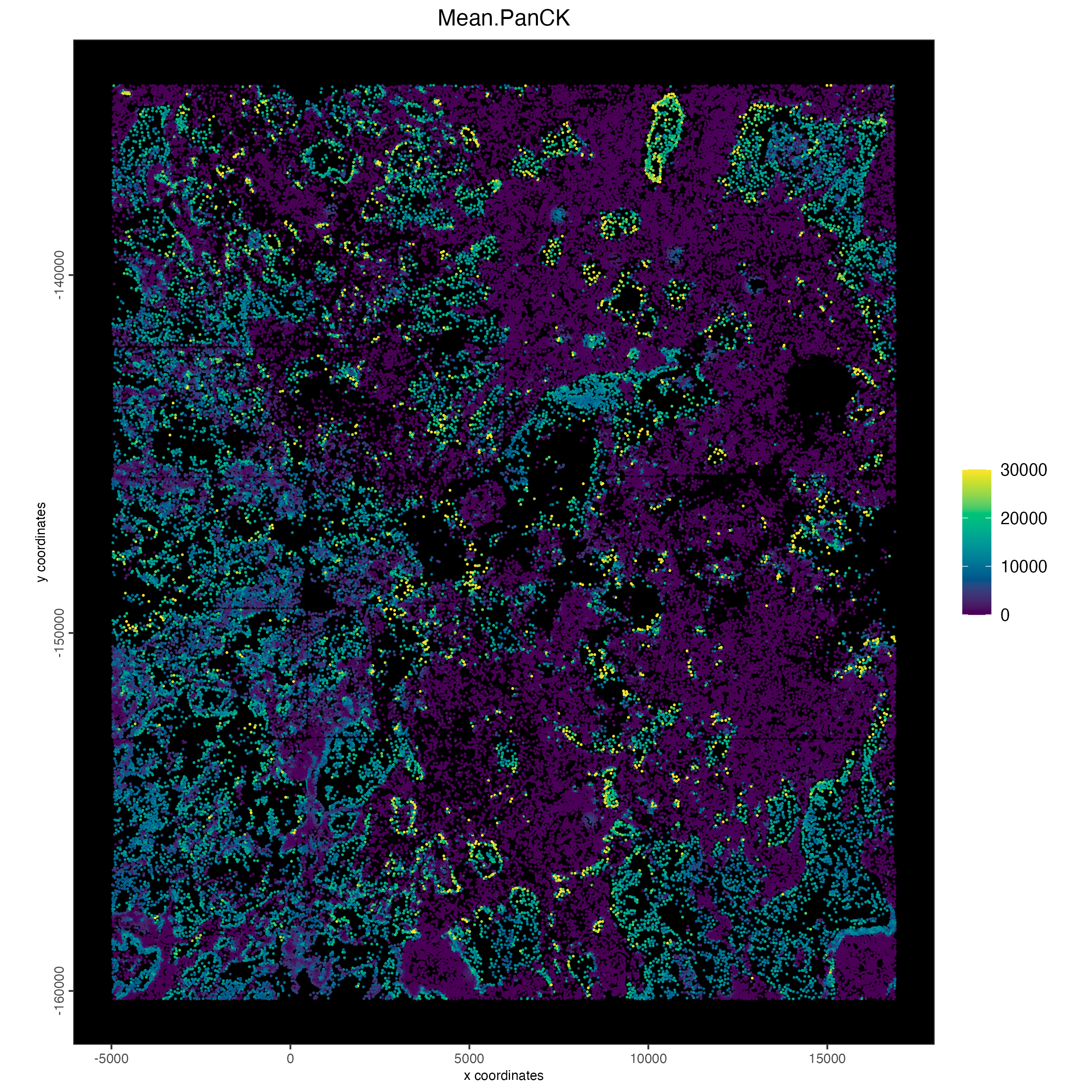
NSCLC is an epithelial cancer, so high expression of cytokeratins are likely cancer.
spatPlot2D(cosmx,
    cell_color = "Mean.PanCK",
    gradient_style = "sequential",
    gradient_limits = c(0, 3e4),
    color_as_factor = FALSE,
    point_border_stroke = 0,
    point_size = 0.8,
    background_color = "black",
    save_param = list(
        save_name = "29_spat_pck"
    )
)
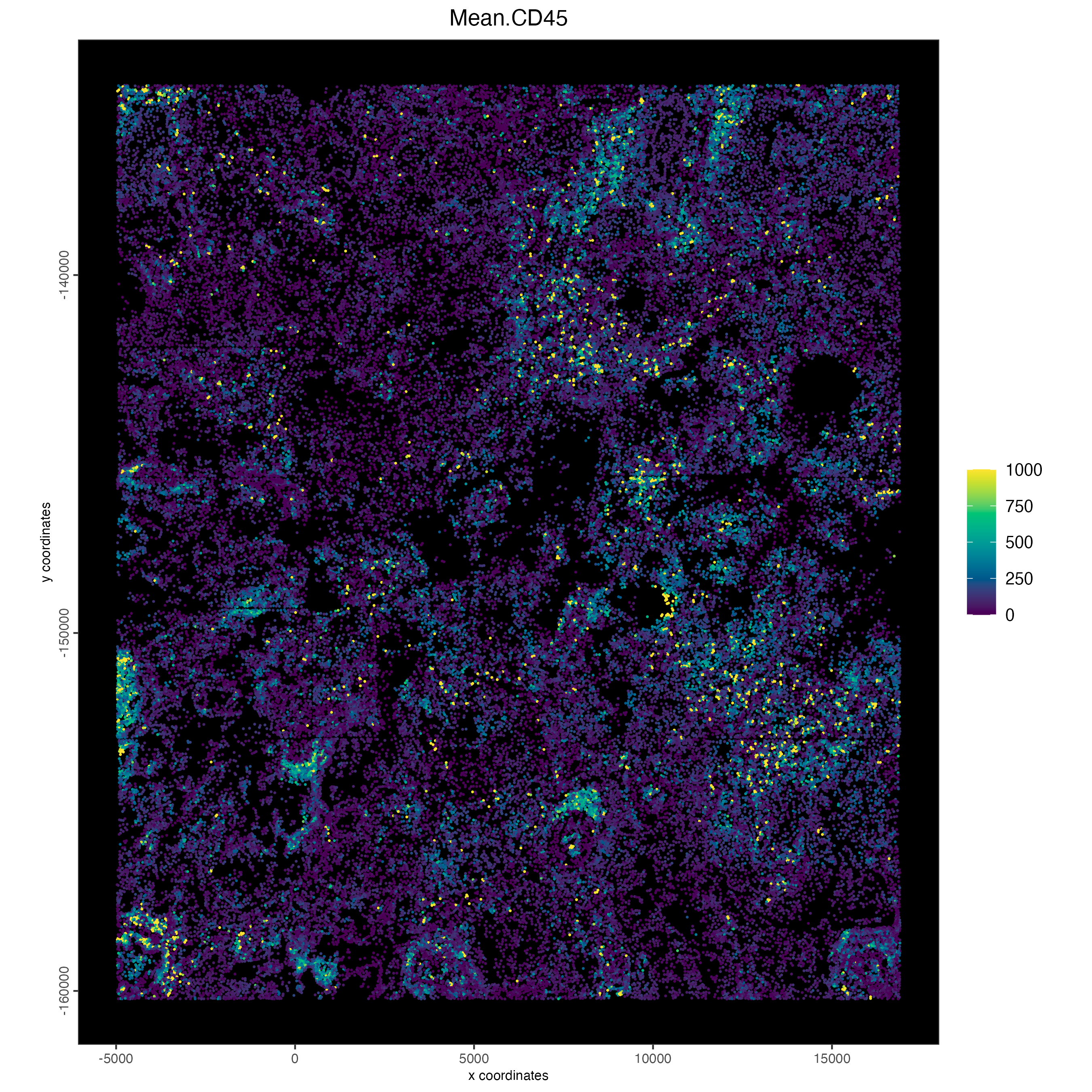
CD45 (general immune marker – T cells, B cells, NK cells, monocytes, macrophages, dendritic cells, and granulocytes)
spatPlot2D(cosmx,
    cell_color = "Mean.CD45",
    gradient_style = "sequential",
    gradient_limits = c(0, 1e3),
    color_as_factor = FALSE,
    point_border_stroke = 0,
    point_size = 0.8,
    background_color = "black",
    save_param = list(
        save_name = "30_spat_cd45"
    )
)
# drop problematic FOV data
p1 <- dimPlot2D(subset(cosmx, subset = !fov %in% c(11,12,14,15,16)),
    cell_color = "Mean.CD3",
    color_as_factor = FALSE,
    cell_color_gradient = custom_scale,
    gradient_limits = c(0, 300),
    point_border_stroke = 0,
    point_size = 0.8,
    show_legend = FALSE,
    background_color = "black",
    return_plot = TRUE,
    save_plot = FALSE
)

p2 <- dimPlot2D(cosmx,
    cell_color = "Mean.PanCK",
    color_as_factor = FALSE,
    cell_color_gradient = custom_scale,
    point_border_stroke = 0,
    point_size = 0.8,
    show_legend = FALSE,
    background_color = "black",
    return_plot = TRUE,
    save_plot = FALSE
)

p3 <- dimPlot2D(cosmx,
    cell_color = "Mean.CD45",
    color_as_factor = FALSE,
    cell_color_gradient = custom_scale,
    gradient_limits = c(0, 1e3),
    point_border_stroke = 0,
    point_size = 0.8,
    show_legend = FALSE,
    background_color = "black",
    return_plot = TRUE,
    save_plot = FALSE
)

stains_plot <- cowplot::plot_grid(p1, p2, p3)
stains_plot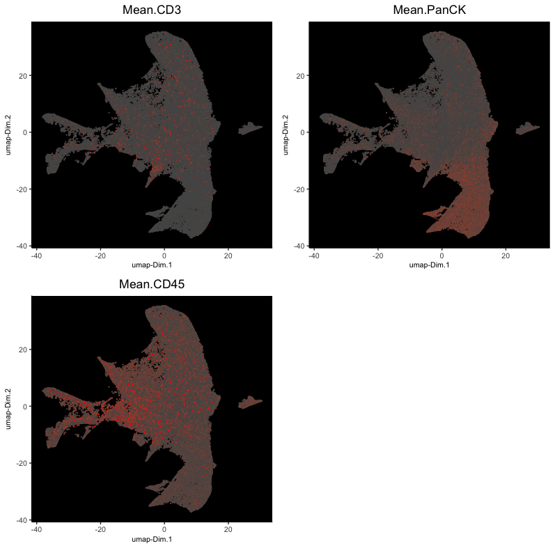
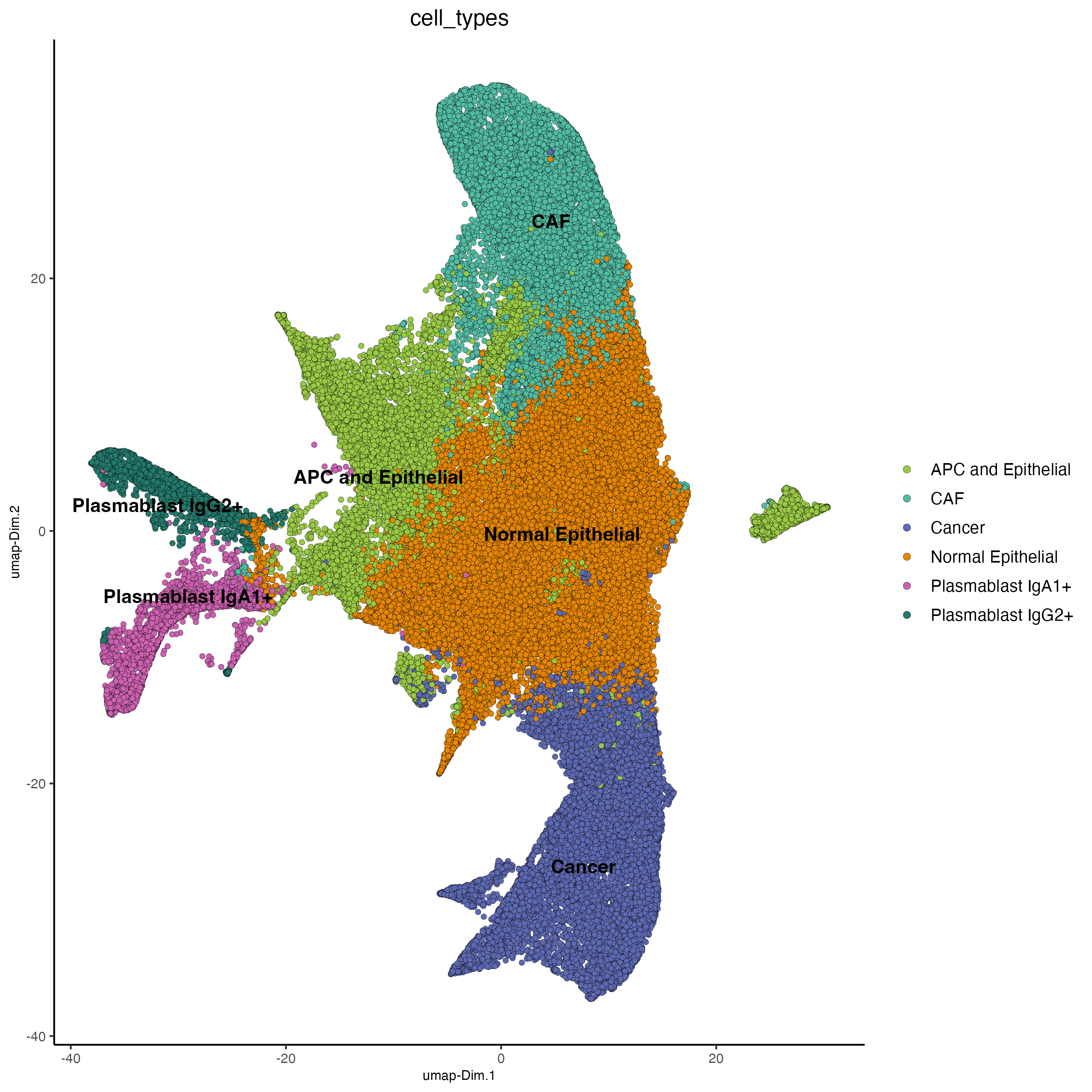
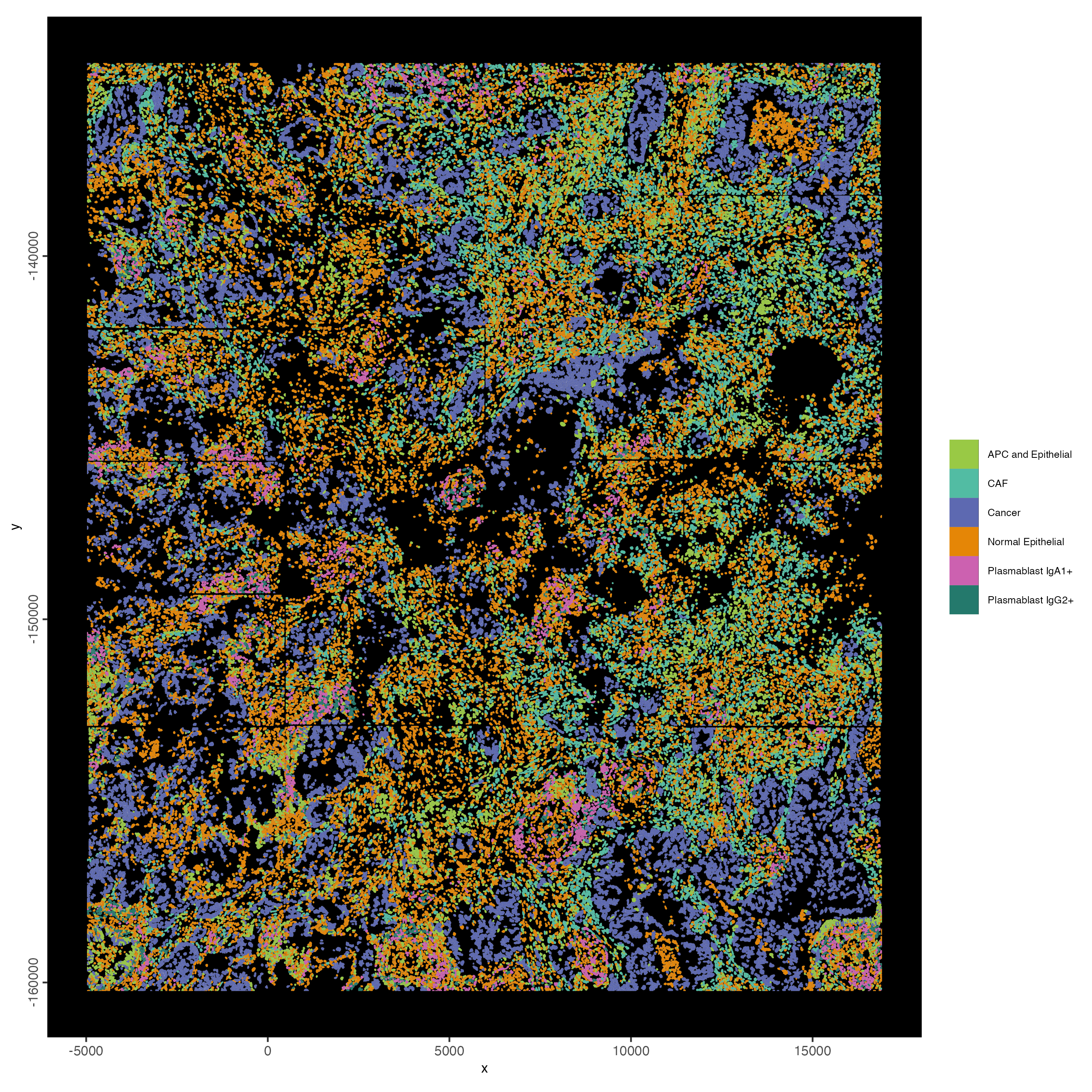
12.5 Cell Type Annotation
## add cell types ###
clusters_cell_types <- c(
    "Normal Epithelial",
    "Cancer",
    "CAF",
    "APC and Epithelial",
    "Plasmablast IgA1+",
    "Plasmablast IgG2+",
    "Normal Epithelial",
    "Plasmablast IgG2+",
    "Plasmablast IgA1+"
)
names(clusters_cell_types) <- seq(9)

ct_colors <- c(
    "CAF" = clus_colors[3],
    "Cancer" = clus_colors[2],
    "Normal Epithelial" = clus_colors[1],
    "APC and Epithelial" = clus_colors[4],
    "Plasmablast IgA1+" = clus_colors[5],
    "Plasmablast IgG2+" = clus_colors[6]
)
Other immune celltypes need further subclustering of leiden clusters 1 and 4. Either that or binarized cutoff approaches might be needed since specific markers for immune celltypes are not cluster specific in this dataset.
cosmx <- annotateGiotto(cosmx,
    annotation_vector = clusters_cell_types,
    cluster_column = "leiden_clus",
    name = "cell_types"
)

plotUMAP(cosmx,
    cell_color = "cell_types",
    cell_color_code = ct_colors,
    point_size = 1.5,
    save_param = list(
        save_name = "32_celltypes_umap"
    )
)
12.6 Visualize
spatInSituPlotPoints(cosmx,
    polygon_fill = "cell_types",
    polygon_fill_code = ct_colors,
    polygon_fill_as_factor = TRUE,
    polygon_line_size = 0.01,
    polygon_color = "white",
    background_color = "black",
    save_param = list(
        save_name = "33_celltypes_sisp"
    )
)
13 Interaction Changed Features (ICF)
Identify features that change based on the proximity of another celltype.
future::plan("multisession", workers = 4) # NOTE: Depending on your system this could take a while
options("future.globals.maxSize" = 1e10)

icf <- findInteractionChangedFeats(cosmx, cluster_column = "cell_types")

# Visualize ICF expression
plotCellProximityFeats(cosmx,
    icfObject = icf,
    method = "dotplot",
    show_plot = FALSE,
    save_plot = TRUE,
    return_plot = FALSE,
    save_param = list(
        save_name = "34_cpf"
    )
)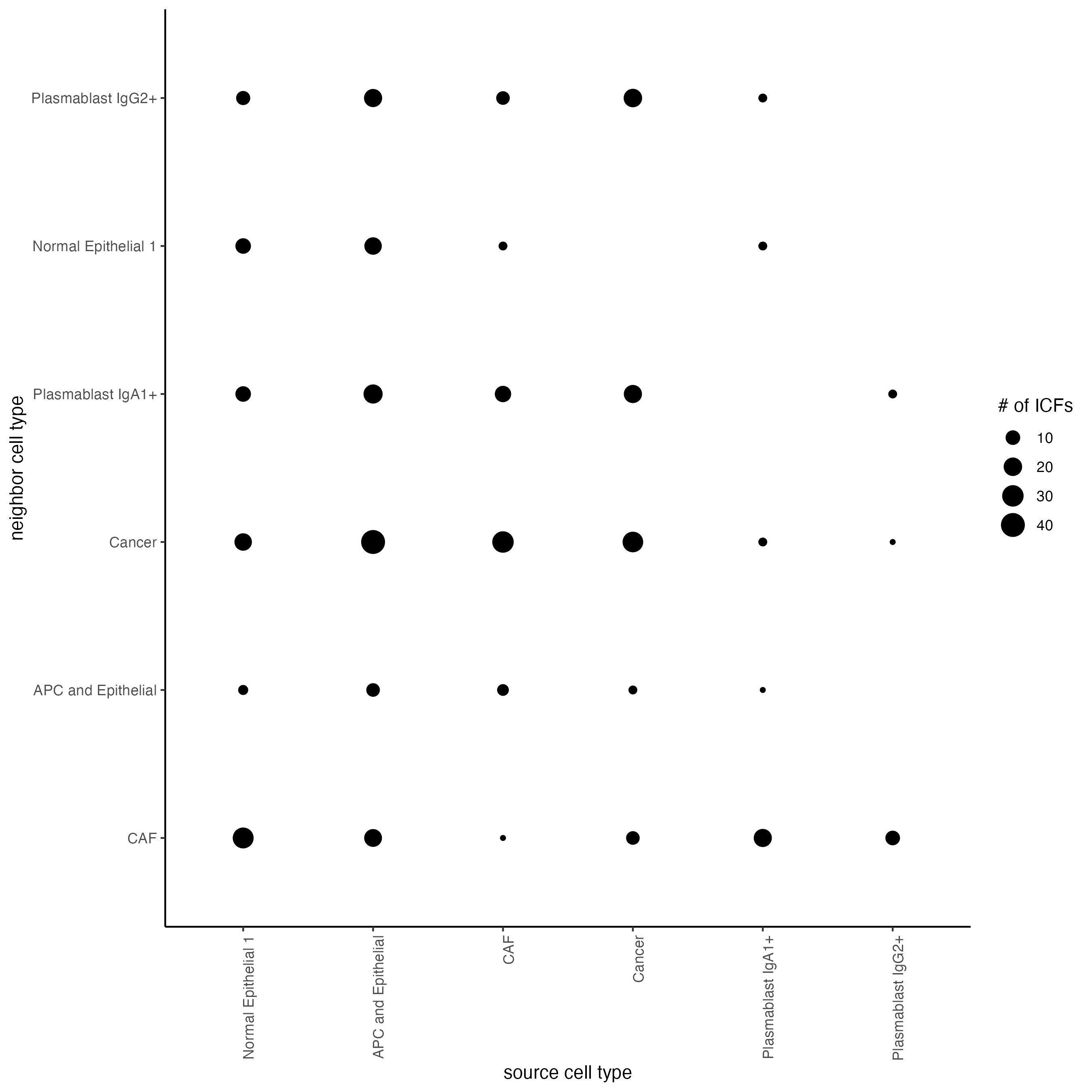
ICF is very sensitive to contaminants, as in transcripts that should belong to another cell, but are mistakenly assigned to your source cell. This is reflected when the top ICFs are celltype markers of the other interacting celltype, instead of a more interesting gene that actually belongs to your source cell that is modulated by the distance to your interacting cell.
icf_filtered <- filterICF(icf,
min_cells = 20,
min_int_cells = 20,
min_fdr = 0.1,
min_spat_diff = 0.1,
min_log2_fc = 0.1,
min_zscore = 1
)
top_icf <- icf_filtered$ICFscores[cell_type == "CAF" & type_int == "hetero", head(.SD, 2), by = int_cell_type]
top_icf_feats <- top_icf$feats
names(top_icf_feats) <- top_icf$int_cell_type
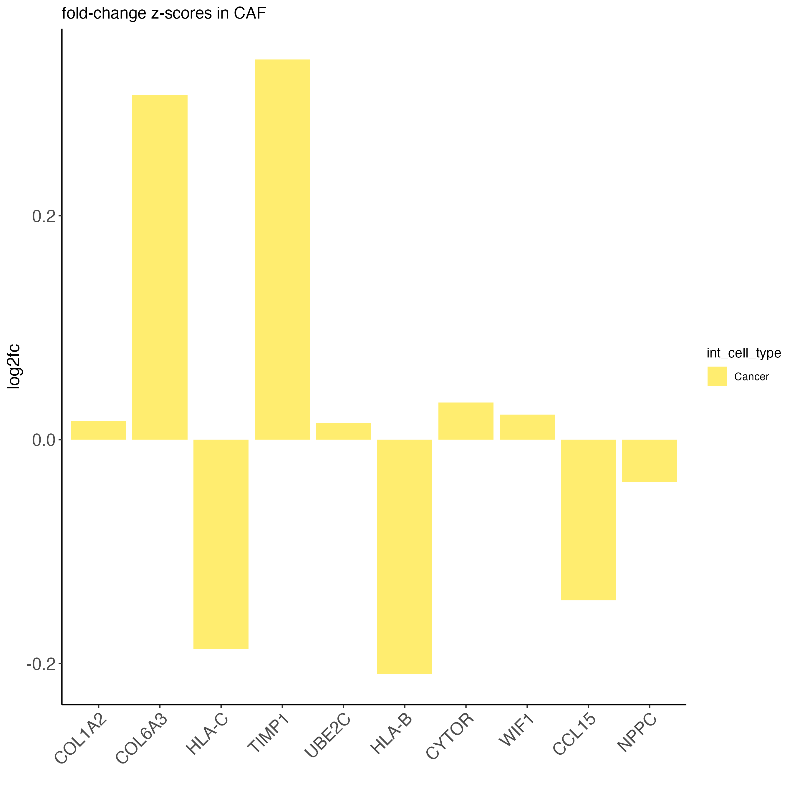
plotICF(cosmx,
icfObject = icf_filtered,
source_type = "CAF",
source_markers = c("COL1A2", "COL6A3"),
ICF_feats = top_icf_feats,
save_param = list(
save_name = "35_icf"
)
)One thing we can do to pick features that that do not have good correlations between their ranks as an icf vs as a marker for the interacting cell type. However, this method of gene selection would have to be repeated for each icf pair of interest.
# find cell type markers
scran_markers <- findMarkers_one_vs_all(cosmx,
    cluster_column = "cell_types",
    min_feats = nrow(cosmx) # do not remove any features
)
scran_markers_Cancer <- scran_markers[cluster == "Cancer"]

# select CAF/Cancer comparison from icfs
icf_table <- icf$ICFscores
icf_table_CAF_cancer <- icf_table[cell_type == "CAF" & int_cell_type == "Cancer"]

# select only shared features between markers and ICFs
cancer_feats <- intersect(scran_markers_Cancer$feats, icf_table$feats)
icf_table_CAF_cancer <- icf_table_CAF_cancer[match(cancer_feats, feats)]
# assign ranks to ICF values
icf_table_CAF_cancer[, rank := seq(.N)]

icf_rank_caf_cancer <- icf_table_CAF_cancer$rank
marker_rank_cancer <- scran_markers_Cancer$ranking

plot(icf_rank_caf_cancer, marker_rank_cancer)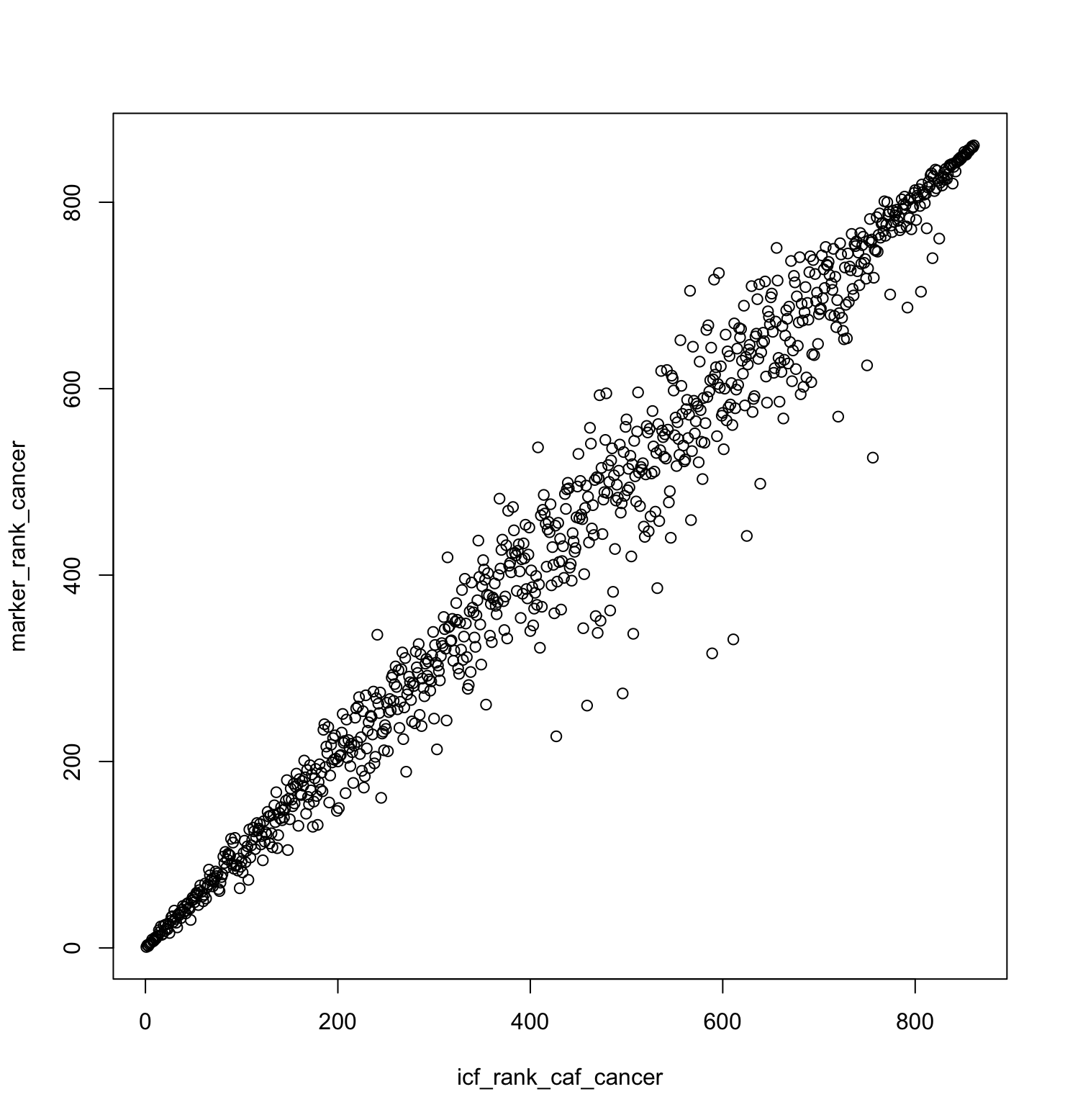
# find differences from the diagonal
center_diffs <- abs(icf_rank_caf_cancer - marker_rank_cancer)
sum(center_diffs > 150) # 8 features greater than 150

# get features to use
cancer_feats_to_use <- cancer_feats[center_diffs > 150]
names(cancer_feats_to_use) <- rep("Cancer", length(cancer_feats_to_use))

plotICF(cosmx,
    icfObject = icf,
    source_type = "CAF",
    source_markers = c("COL1A2", "COL6A3"),
    ICF_feats = cancer_feats_to_use,
    save_param = list(
        save_name = "37_caf_cancer_icf"
    )
)
14 Saving the giotto object
Giotto uses many objects that include pointers to information that
live on disk instead of loading everything into memory. This includes
both giotto image objects (giottoImage,
giottoLargeImage) and also subcellular information
(giottoPoints, giottoPolygon). When saving the
project as a .RDS or .Rdata, these pointers
are broken and can produce errors when loaded again.
saveGiotto() is a function that can save Giotto Suite
projects into a contained structured directory that can then be properly
loaded again later using loadGiotto().
saveGiotto(gobject = fov_join,
           export_image = FALSE, # don't save the images again, and rely on reconnections
           foldername = "new_folder_name",
           dir = "/directory/to/save/to/")
15 Session Info
R version 4.4.1 (2024-06-14)
Platform: aarch64-apple-darwin20
Running under: macOS 15.0.1

Matrix products: default
BLAS:   /System/Library/Frameworks/Accelerate.framework/Versions/A/Frameworks/vecLib.framework/Versions/A/libBLAS.dylib
LAPACK: /Library/Frameworks/R.framework/Versions/4.4-arm64/Resources/lib/libRlapack.dylib;  LAPACK version 3.12.0

locale:
[1] en_US.UTF-8/en_US.UTF-8/en_US.UTF-8/C/en_US.UTF-8/en_US.UTF-8

time zone: America/New_York
tzcode source: internal

attached base packages:
[1] stats     graphics  grDevices utils     datasets  methods   base

other attached packages:
[1] Giotto_4.2.0      GiottoClass_0.4.6

loaded via a namespace (and not attached):
  [1] colorRamp2_0.1.0            deldir_2.0-4                rlang_1.1.4
  [4] magrittr_2.0.3              RcppAnnoy_0.0.22            GiottoUtils_0.2.3
  [7] matrixStats_1.4.1           compiler_4.4.1              png_0.1-8
 [10] systemfonts_1.1.0           vctrs_0.6.5                 pkgconfig_2.0.3
 [13] SpatialExperiment_1.14.0    crayon_1.5.3                fastmap_1.2.0
 [16] backports_1.5.0             magick_2.8.5                XVector_0.44.0
 [19] labeling_0.4.3              utf8_1.2.4                  rmarkdown_2.29
 [22] UCSC.utils_1.0.0            ragg_1.3.2                  purrr_1.0.2
 [25] xfun_0.49                   zlibbioc_1.50.0             beachmat_2.20.0
 [28] GenomeInfoDb_1.40.0         jsonlite_1.8.9              DelayedArray_0.30.0
 [31] BiocParallel_1.38.0         terra_1.7-78                irlba_2.3.5.1
 [34] parallel_4.4.1              R6_2.5.1                    RColorBrewer_1.1-3
 [37] reticulate_1.39.0           parallelly_1.38.0           rcartocolor_2.1.1
 [40] GenomicRanges_1.56.0        scattermore_1.2             Rcpp_1.0.13-1
 [43] SummarizedExperiment_1.34.0 knitr_1.49                  future.apply_1.11.2
 [46] R.utils_2.12.3              IRanges_2.38.0              Matrix_1.7-0
 [49] igraph_2.1.1                tidyselect_1.2.1            yaml_2.3.10
 [52] rstudioapi_0.16.0           abind_1.4-8                 codetools_0.2-20
 [55] listenv_0.9.1               lattice_0.22-6              tibble_3.2.1
 [58] Biobase_2.64.0              withr_3.0.2                 Rtsne_0.17
 [61] evaluate_1.0.1              future_1.34.0               pillar_1.9.0
 [64] MatrixGenerics_1.16.0       checkmate_2.3.2             stats4_4.4.1
 [67] dbscan_1.2-0                plotly_4.10.4               generics_0.1.3
 [70] S4Vectors_0.42.0            ggplot2_3.5.1               munsell_0.5.1
 [73] scales_1.3.0                gtools_3.9.5                globals_0.16.3
 [76] glue_1.8.0                  lazyeval_0.2.2              tools_4.4.1
 [79] GiottoVisuals_0.2.11        data.table_1.16.2           ScaledMatrix_1.12.0
 [82] cowplot_1.1.3               grid_4.4.1                  tidyr_1.3.1
 [85] colorspace_2.1-1            SingleCellExperiment_1.26.0 GenomeInfoDbData_1.2.12
 [88] BiocSingular_1.20.0         cli_3.6.3                   rsvd_1.0.5
 [91] textshaping_0.3.7           fansi_1.0.6                 S4Arrays_1.4.0
 [94] viridisLite_0.4.2           dplyr_1.1.4                 uwot_0.2.2
 [97] gtable_0.3.6                R.methodsS3_1.8.2           digest_0.6.37
[100] progressr_0.14.0            BiocGenerics_0.50.0         SparseArray_1.4.1
[103] ggrepel_0.9.6               rjson_0.2.21                htmlwidgets_1.6.4
[106] farver_2.1.2                R.oo_1.26.0                 htmltools_0.5.8.1
[109] lifecycle_1.0.4             httr_1.4.7