10X Single Cell RNA Sequencing
Source:vignettes/singlecell_prostate_standard.Rmd
singlecell_prostate_standard.Rmd1 Dataset Explanation
Ma et al. Processed 10X Single Cell RNAseq from two prostate cancer patients. The raw dataset can be found here. To run this tutorial we will use the sample 1.
2 Set up Giotto Environment
# Ensure Giotto Suite is installed.
if(!"Giotto" %in% installed.packages()) {
  pak::pkg_install("drieslab/Giotto")
}

# Ensure the Python environment for Giotto has been installed.
genv_exists <- Giotto::checkGiottoEnvironment()
if(!genv_exists){
  # The following command need only be run once to install the Giotto environment.
  Giotto::installGiottoEnvironment()
}
library(Giotto)

# 1. set working directory
results_folder <- "/path/to/results/"

# Optional: Specify a path to a Python executable within a conda or miniconda
# environment. If set to NULL (default), the Python executable within the previously
# installed Giotto environment will be used.
python_path <- NULL # alternatively, "/local/python/path/python" if desired.

# 3. create giotto instructions
instructions <- createGiottoInstructions(save_dir = results_folder,
                                         save_plot = TRUE,
                                         show_plot = FALSE,
                                         python_path = python_path)
3 Create Giotto object from 10X dataset
Note that you will need an input directory for barcodes.tsv(.gz) features.tsv(.gz) matrix.mtx(.gz)
data_path <- "/path/to/data/"

expression <- read.table(paste0(data_path, "GSM4773521_PCa1_gene_counts_matrix.txt"))

giotto_SC <- createGiottoObject(expression = expression,
                                instructions = instructions)
4 Process Giotto Object
giotto_SC <- filterGiotto(gobject = giotto_SC,
                          expression_threshold = 1,
                          feat_det_in_min_cells = 50,
                          min_det_feats_per_cell = 500,
                          expression_values = "raw",
                          verbose = TRUE)

## normalize
giotto_SC <- normalizeGiotto(gobject = giotto_SC,
                             scalefactor = 6000)

## add mitochondria gene percentage and filter giotto object by percent mito
library(rtracklayer)

## run wget http://ftp.ensembl.org/pub/release-105/gtf/homo_sapiens/Homo_sapiens.GRCh38.105.gtf.gz

gtf <- import("Homo_sapiens.GRCh38.105.gtf.gz")
gtf <- gtf[gtf$gene_name!="" & !is.na(gtf$gene_name)]
mito <- gtf$gene_name[as.character(seqnames(gtf)) %in% "MT"]
mito <- unique(mito)

giotto_SC <- addFeatsPerc(giotto_SC,
                          feats = mito,
                          vector_name = "perc_mito")

giotto_SC <- subsetGiotto(giotto_SC,
                          cell_ids = pDataDT(giotto_SC)[which(pDataDT(giotto_SC)$perc_mito < 15),]$cell_ID)


## add gene & cell statistics
giotto_SC <- addStatistics(gobject = giotto_SC,
                           expression_values = "raw")
5 Dimension Reduction
## PCA ##
giotto_SC <- calculateHVF(gobject = giotto_SC)

giotto_SC <- runPCA(gobject = giotto_SC,
                    center = TRUE,
                    scale_unit = TRUE)

screePlot(giotto_SC,
          ncp = 30,
          save_param = list(save_name = "3_scree_plot"))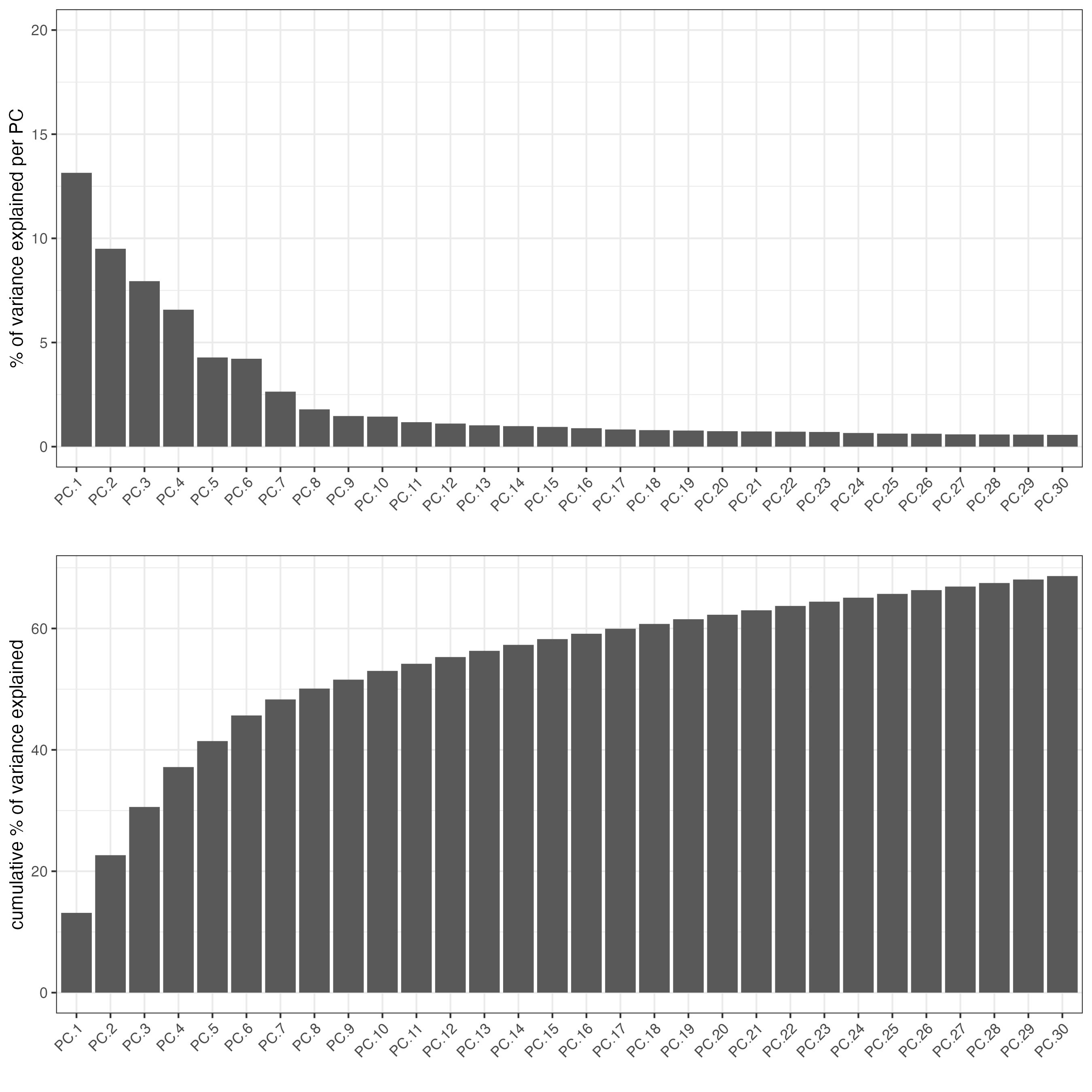
6 Cluster
## cluster and run UMAP ##
# sNN network (default)
showGiottoDimRed(giotto_SC)

giotto_SC <- createNearestNetwork(gobject = giotto_SC,
                                  dim_reduction_to_use = "pca",
                                  dim_reduction_name = "pca",
                                  dimensions_to_use = 1:10,
                                  k = 15)

# UMAP
giotto_SC <- runUMAP(giotto_SC,
                     dimensions_to_use = 1:10)

# Leiden clustering
giotto_SC <- doLeidenCluster(gobject = giotto_SC,
                             resolution = 0.2,
                             n_iterations = 1000)

plotUMAP(gobject = giotto_SC,
         cell_color = "leiden_clus",
         show_NN_network = TRUE,
         point_size = 1.5,
         save_param = list(save_name = "4_Cluster"))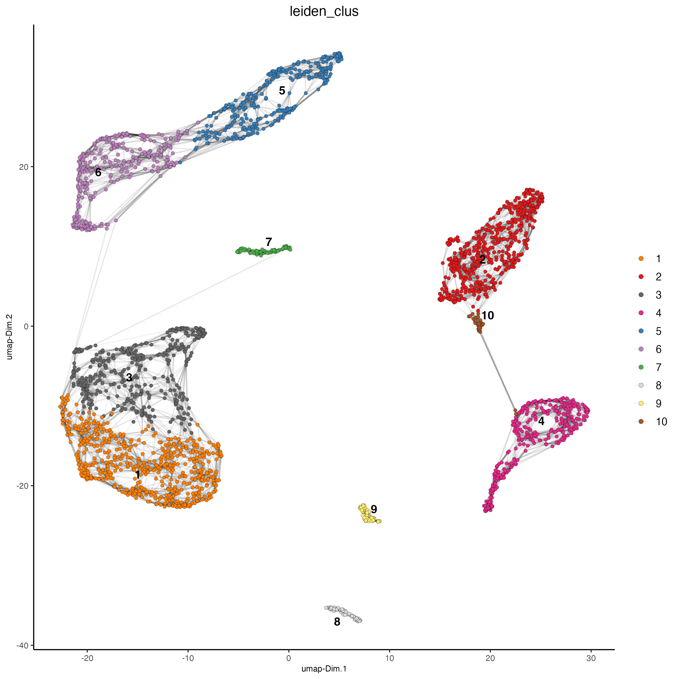
7 Differential Expression
markers_scran <- findMarkers_one_vs_all(gobject = giotto_SC,
                                       method = "scran",
                                       expression_values = "normalized",
                                       cluster_column = "leiden_clus",
                                       min_feats = 3)

topgenes_scran <- unique(markers_scran[, head(.SD, 3), by = "cluster"][["feats"]])

plotMetaDataHeatmap(giotto_SC,
                    expression_values = "normalized",
                    metadata_cols = "leiden_clus",
                    selected_feats = topgenes_scran,
                    y_text_size = 8,
                    show_values = "zscores_rescaled",
                    save_param = list(save_name = "5_a_metaheatmap"))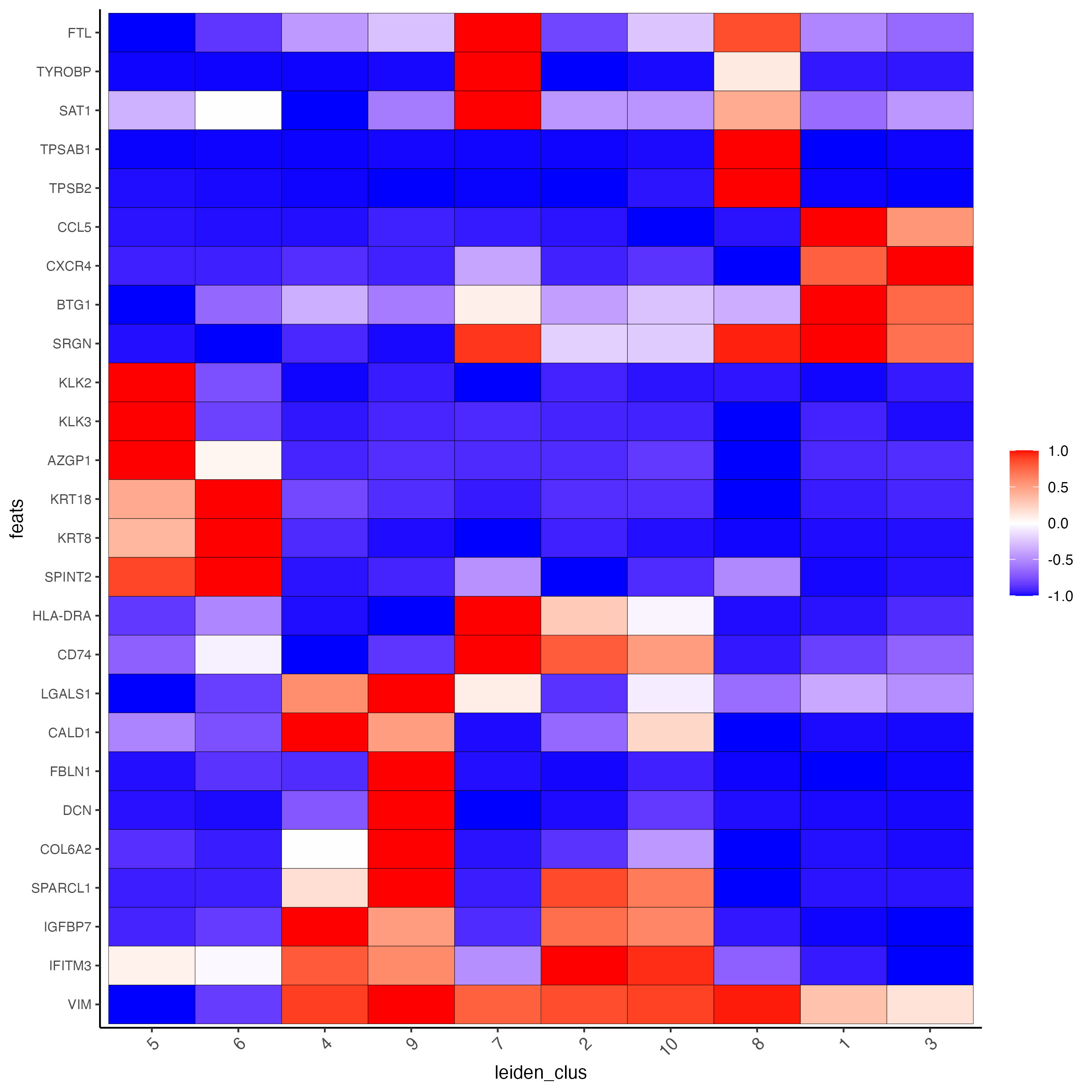
topgenes_scran <- markers_scran[, head(.SD, 1), by = "cluster"]$feats

# violinplot
violinPlot(giotto_SC,
           feats = unique(topgenes_scran),
           cluster_column = "leiden_clus",
           strip_text = 10,
           strip_position = "right",
           save_param = list(save_name = "5_b_violinplot_scran", base_width = 5))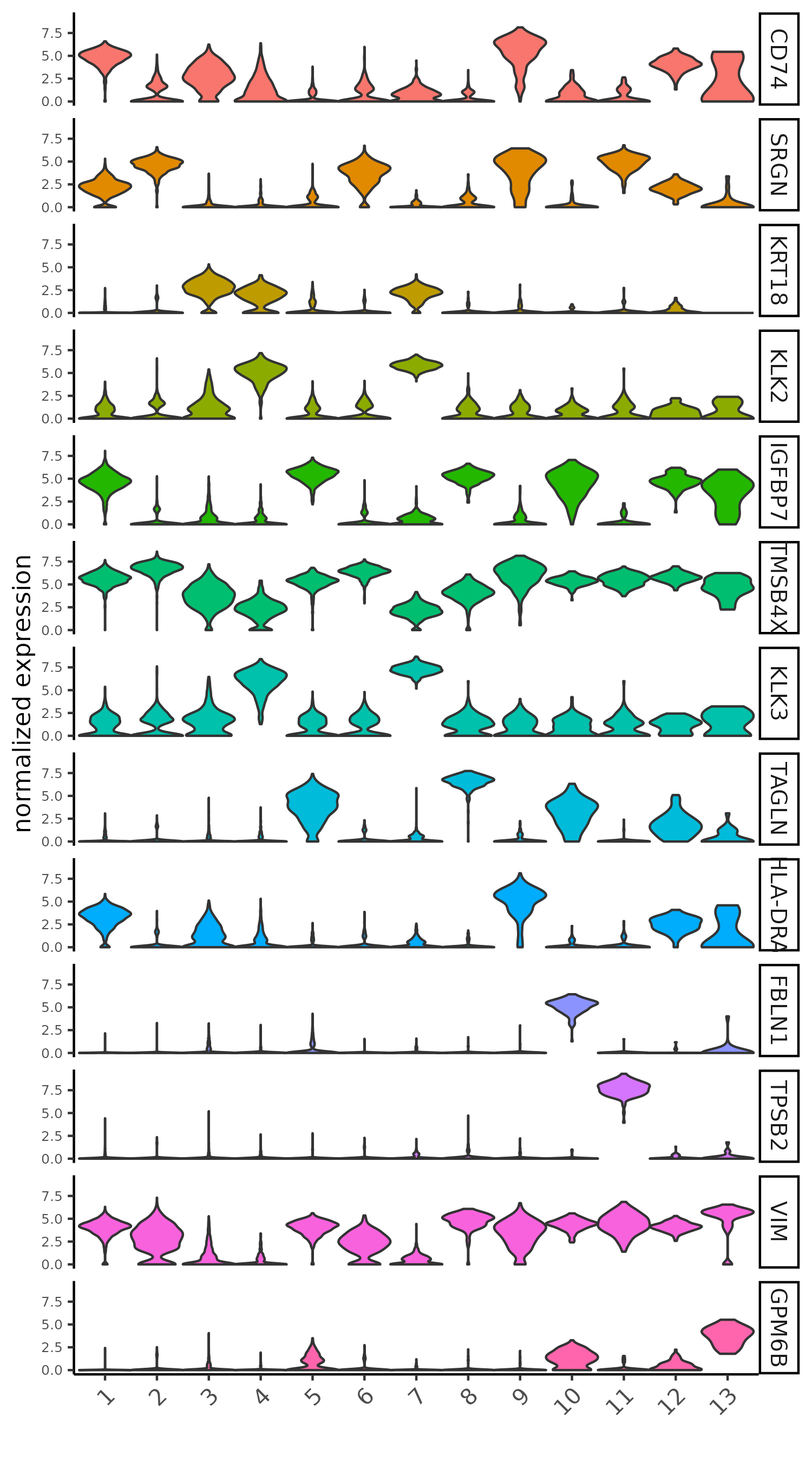
8 FeaturePlot
# Plot known marker genes across different cell types. EPCAM for epithelial cells,
# DPP4(CD26) for Epithelial luminal cells, PECAM1(CD31) for Endothelial cells and CD3D for T cells
dimFeatPlot2D(giotto_SC,
              feats = c("EPCAM","DPP4","PECAM1","CD3D"),
              cow_n_col = 2,
              save_param = list(save_name = "6_featureplot"))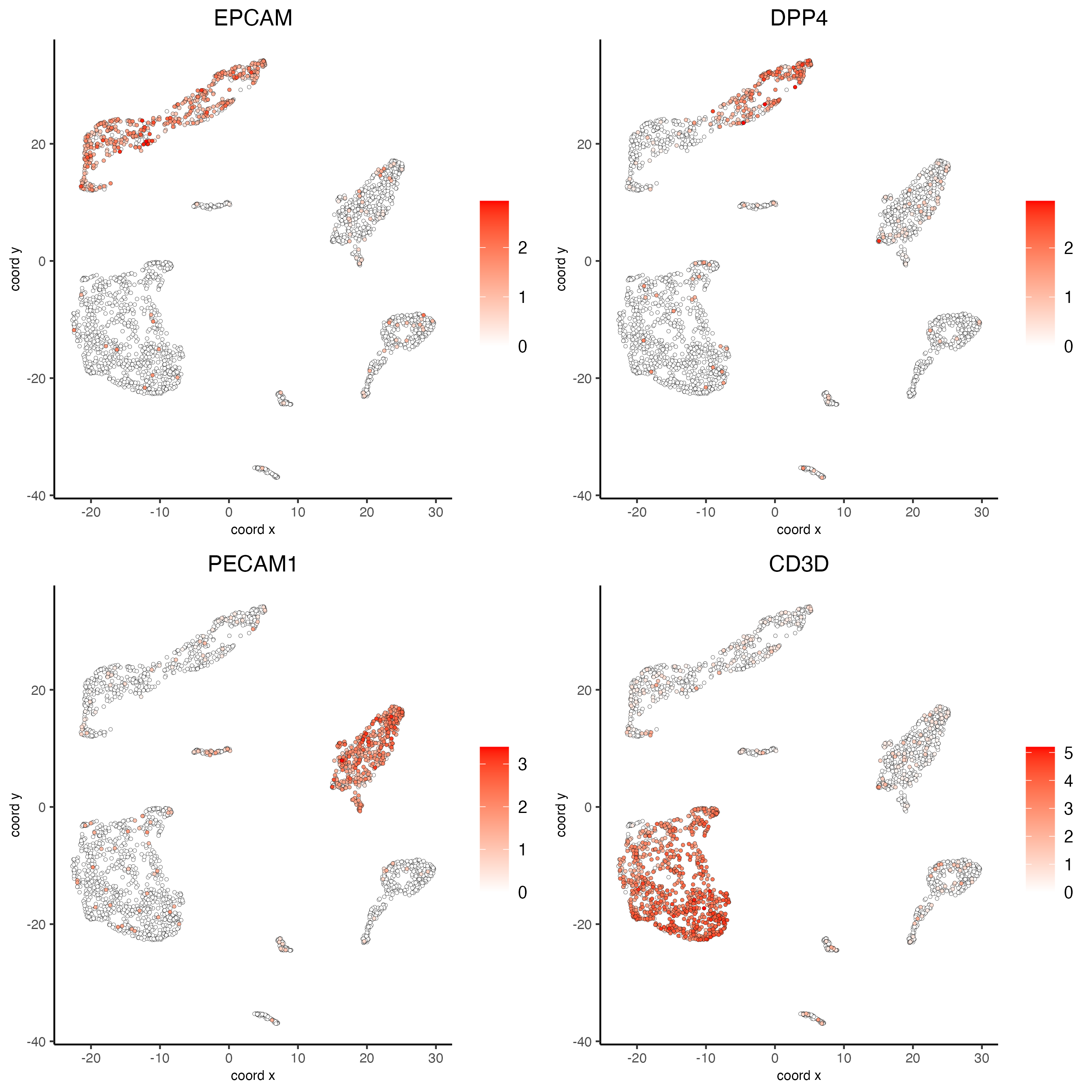
9 Cell type Annotation
prostate_labels <- c("Endothelial cells",#1
                     "T cells",#2
                     "Epithelial_basal",#3
                     "Epithelial_luminal",#4
                     "Fibroblasts",#5
                     "T cells",#6
                     "Epithelial_luminal",#7
                     "Smooth muscle cells",#8
                     "Macrophage & B cells",#9
                     "Fibroblasts",#10
                     "Mast cells",#11
                     "Mesenchymal cells",#12
                     "Neural Progenitor cells")#13

names(prostate_labels) <- 1:13

giotto_SC <- annotateGiotto(gobject = giotto_SC,
                            annotation_vector = prostate_labels,
                            cluster_column = "leiden_clus",
                            name = "prostate_labels")

dimPlot2D(gobject = giotto_SC,
          dim_reduction_name = "umap",
          cell_color = "prostate_labels",
          show_NN_network = TRUE,
          point_size = 1.5,
          save_param = list(save_name = "7_Annotation"))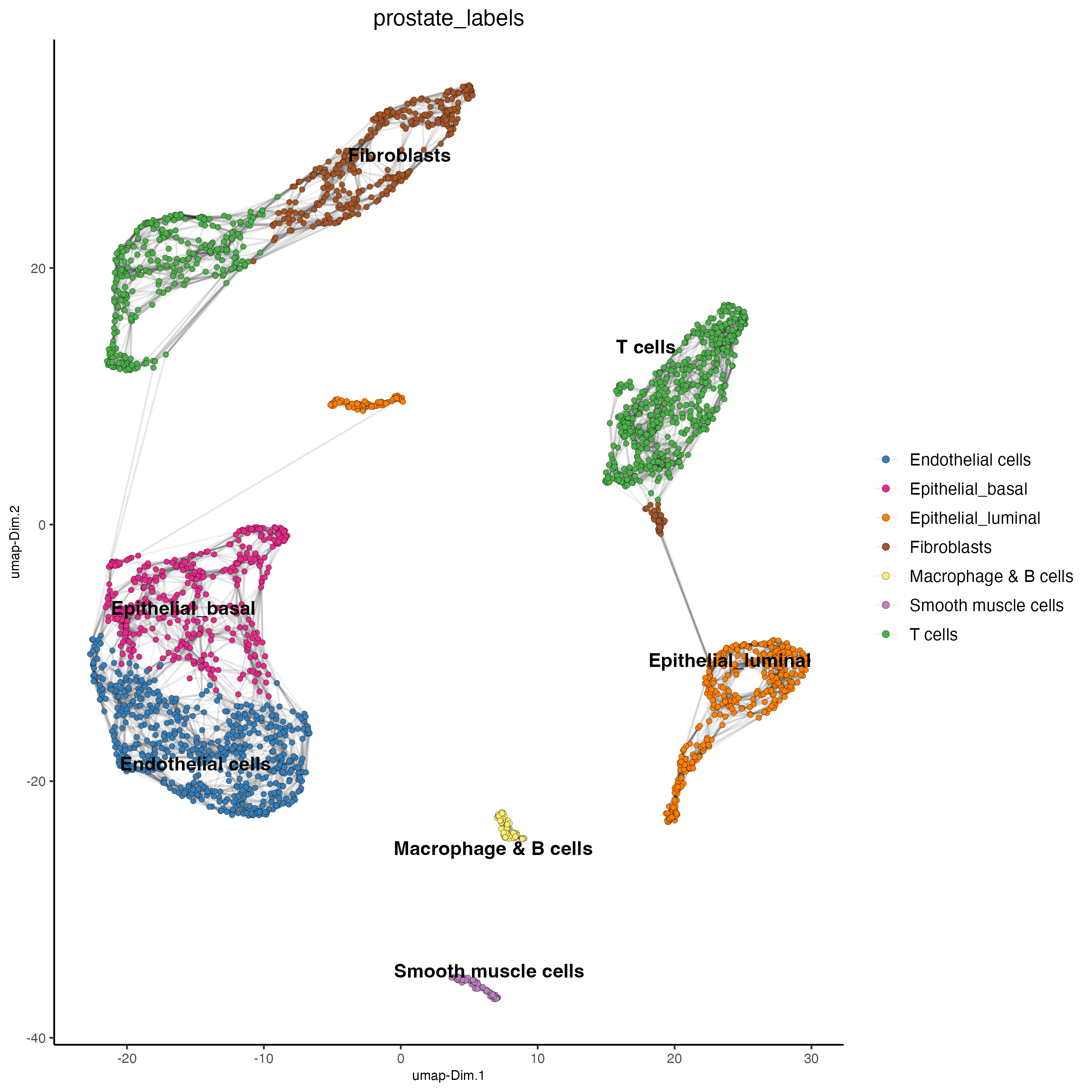
10 Subset and Recluster
Subset_giotto_T <- subsetGiotto(giotto_SC,
                                cell_ids = pDataDT(giotto_SC)[which(pDataDT(giotto_SC)$prostate_labels == "T cells"),]$cell_ID)

## PCA
Subset_giotto_T <- calculateHVF(gobject = Subset_giotto_T)

Subset_giotto_T <- runPCA(gobject = Subset_giotto_T,
                          center = TRUE,
                          scale_unit = TRUE)

screePlot(Subset_giotto_T,
          ncp = 20,
          save_param = list(save_name = "8a_scree_plot"))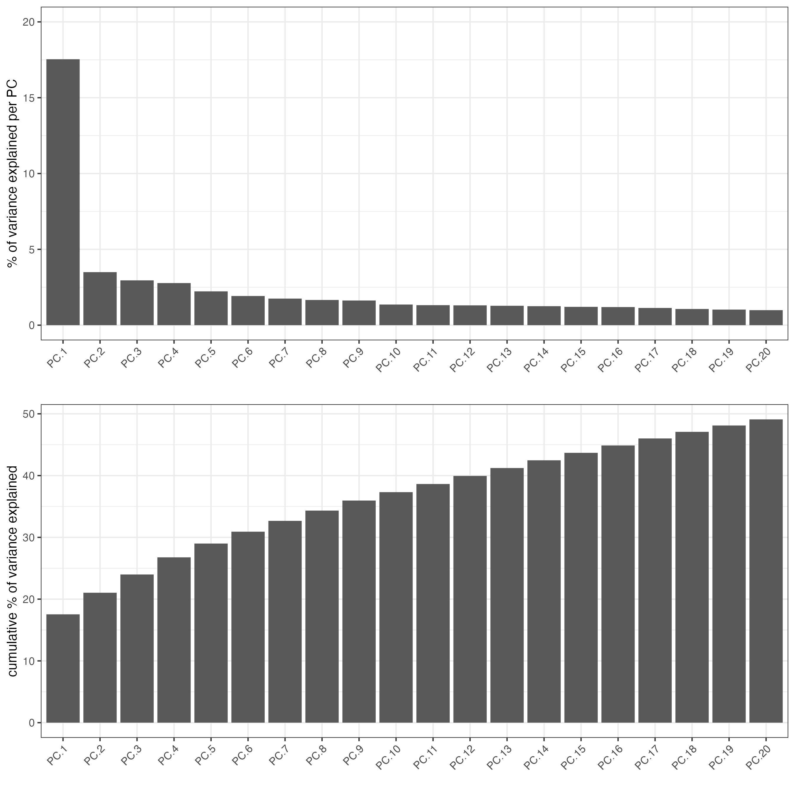
Subset_giotto_T <- createNearestNetwork(gobject = Subset_giotto_T,
                                        dim_reduction_to_use = "pca",
                                        dim_reduction_name = "pca",
                                        dimensions_to_use = 1:20,
                                        k = 10)

# UMAP
Subset_giotto_T <- runUMAP(Subset_giotto_T,
                           dimensions_to_use = 1:8)

# Leiden clustering
Subset_giotto_T <- doLeidenCluster(gobject = Subset_giotto_T,
                                   resolution = 0.1,
                                   n_iterations = 1000)


plotUMAP(gobject = Subset_giotto_T,
         cell_color = "leiden_clus",
         show_NN_network = TRUE,
         point_size = 1.5,
         save_param = list(save_name = "8b_Cluster"))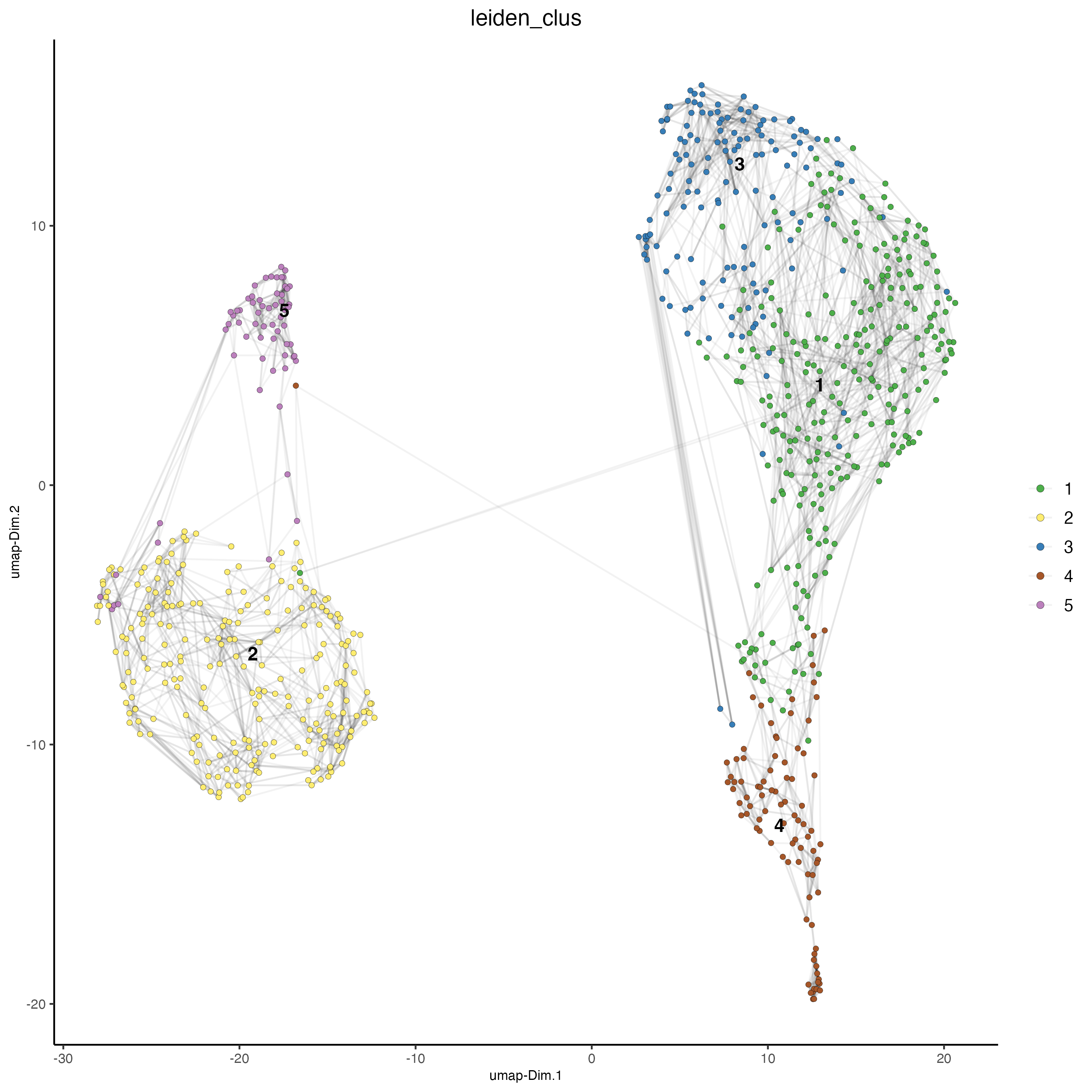
markers_scran_T = findMarkers_one_vs_all(gobject=Subset_giotto_T,
                                         method = "scran",
                                         expression_values = "normalized",
                                         cluster_column = "leiden_clus",
                                         min_feats = 3)

topgenes_scran_T <- unique(markers_scran_T[, head(.SD, 5), by = "cluster"][["feats"]])

plotMetaDataHeatmap(Subset_giotto_T,
                    expression_values = "normalized",
                    metadata_cols = "leiden_clus",
                    selected_feats = topgenes_scran_T,
                    y_text_size = 8,
                    show_values = "zscores_rescaled",
                    save_param = list(save_name = "8_c_metaheatmap"))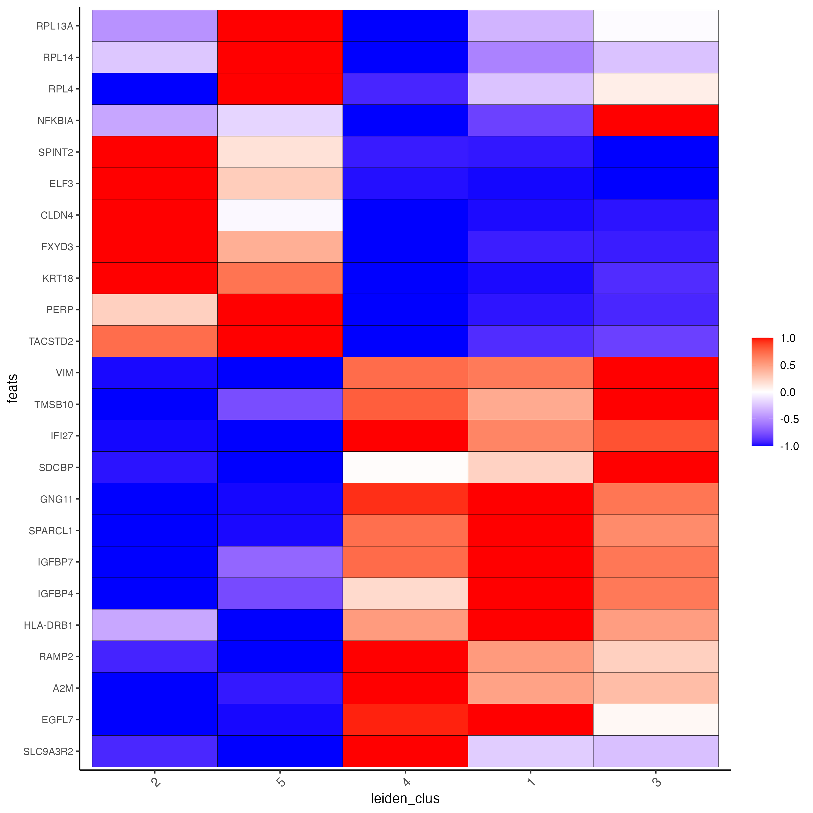
T_labels <- c("Naive T cells",#1
              "Tfh cells",#2
              "CD8 T cells",#3
              "NK T cells",#4
              "CD4 T cells")#5

names(T_labels) <- 1:5

Subset_giotto_T <- annotateGiotto(gobject = Subset_giotto_T,
                                  annotation_vector = T_labels,
                                  cluster_column = "leiden_clus",
                                  name = "subset_labels")

dimPlot2D(gobject = Subset_giotto_T,
          dim_reduction_name = "umap",
          cell_color = "subset_labels",
          show_NN_network = TRUE,
          point_size = 1.5,
          save_param = list(save_name = "8d_Annotation"))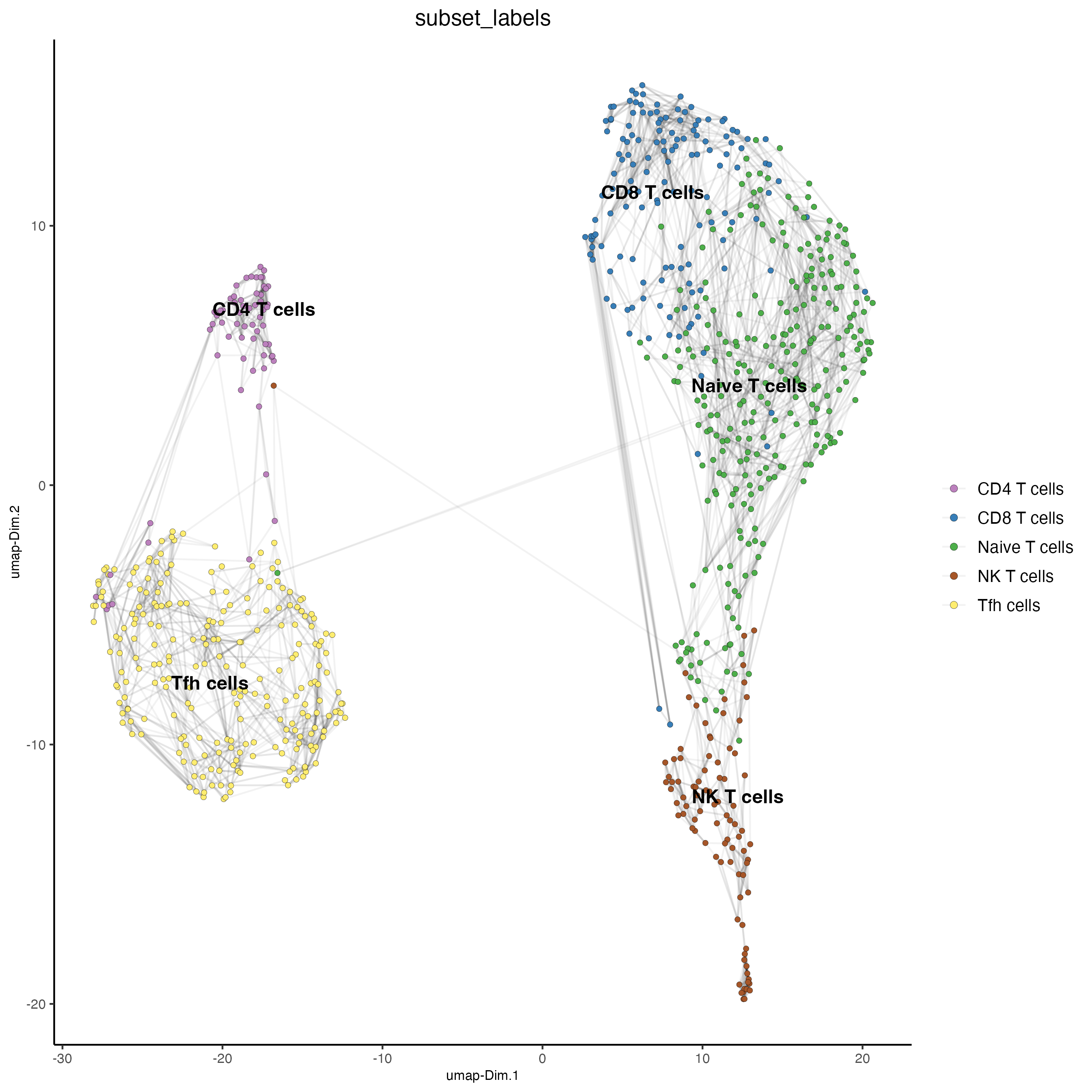
11 Session Info
R version 4.3.2 (2023-10-31)
Platform: aarch64-apple-darwin20 (64-bit)
Running under: macOS Sonoma 14.2.1

Matrix products: default
BLAS:   /System/Library/Frameworks/Accelerate.framework/Versions/A/Frameworks/vecLib.framework/Versions/A/libBLAS.dylib
LAPACK: /Library/Frameworks/R.framework/Versions/4.3-arm64/Resources/lib/libRlapack.dylib;  LAPACK version 3.11.0

locale:
[1] en_US.UTF-8/en_US.UTF-8/en_US.UTF-8/C/en_US.UTF-8/en_US.UTF-8

time zone: America/New_York
tzcode source: internal

attached base packages:
[1] stats4    stats     graphics  grDevices utils     datasets  methods   base

other attached packages:
[1] rtracklayer_1.62.0   GenomicRanges_1.54.1 GenomeInfoDb_1.38.6  IRanges_2.36.0
[5] S4Vectors_0.40.2     BiocGenerics_0.48.1  Giotto_4.0.3         GiottoClass_0.1.3

loaded via a namespace (and not attached):
  [1] colorRamp2_0.1.0            bitops_1.0-7                rlang_1.1.3
  [4] magrittr_2.0.3              GiottoUtils_0.1.5           matrixStats_1.2.0
  [7] compiler_4.3.2              DelayedMatrixStats_1.24.0   png_0.1-8
 [10] systemfonts_1.0.5           vctrs_0.6.5                 pkgconfig_2.0.3
 [13] SpatialExperiment_1.12.0    crayon_1.5.2                fastmap_1.1.1
 [16] backports_1.4.1             magick_2.8.3                XVector_0.42.0
 [19] scuttle_1.12.0              labeling_0.4.3              utf8_1.2.4
 [22] Rsamtools_2.18.0            rmarkdown_2.25              ragg_1.2.7
 [25] bluster_1.12.0              xfun_0.42                   zlibbioc_1.48.0
 [28] beachmat_2.18.1             jsonlite_1.8.8              DelayedArray_0.28.0
 [31] BiocParallel_1.36.0         terra_1.7-71                cluster_2.1.6
 [34] irlba_2.3.5.1               parallel_4.3.2              R6_2.5.1
 [37] RColorBrewer_1.1-3          limma_3.58.1                reticulate_1.35.0
 [40] parallelly_1.37.0           Rcpp_1.0.12                 SummarizedExperiment_1.32.0
 [43] knitr_1.45                  future.apply_1.11.1         FNN_1.1.4
 [46] Matrix_1.6-5                igraph_2.0.2                tidyselect_1.2.0
 [49] rstudioapi_0.15.0           abind_1.4-5                 yaml_2.3.8
 [52] codetools_0.2-19            listenv_0.9.1               lattice_0.22-5
 [55] tibble_3.2.1                Biobase_2.62.0              withr_3.0.0
 [58] evaluate_0.23               future_1.33.1               Biostrings_2.70.2
 [61] pillar_1.9.0                MatrixGenerics_1.14.0       checkmate_2.3.1
 [64] generics_0.1.3              dbscan_1.1-12               RCurl_1.98-1.14
 [67] ggplot2_3.4.4               sparseMatrixStats_1.14.0    munsell_0.5.0
 [70] scales_1.3.0                gtools_3.9.5                globals_0.16.2
 [73] glue_1.7.0                  metapod_1.10.1              tools_4.3.2
 [76] GiottoVisuals_0.1.4         BiocIO_1.12.0               BiocNeighbors_1.20.2
 [79] data.table_1.15.0           ScaledMatrix_1.10.0         locfit_1.5-9.8
 [82] GenomicAlignments_1.38.2    scran_1.30.2                XML_3.99-0.16.1
 [85] cowplot_1.1.3               grid_4.3.2                  edgeR_4.0.15
 [88] colorspace_2.1-0            SingleCellExperiment_1.24.0 GenomeInfoDbData_1.2.11
 [91] BiocSingular_1.18.0         restfulr_0.0.15             cli_3.6.2
 [94] rsvd_1.0.5                  textshaping_0.3.7           fansi_1.0.6
 [97] S4Arrays_1.2.0              dplyr_1.1.4                 uwot_0.1.16
[100] gtable_0.3.4                digest_0.6.34               progressr_0.14.0
[103] dqrng_0.3.2                 SparseArray_1.2.4           ggrepel_0.9.5
[106] rjson_0.2.21                farver_2.1.1                htmltools_0.5.7
[109] lifecycle_1.0.4             statmod_1.5.0