Multi-omics spatial RNA-ATAC seq Mouse Embryo
Source:vignettes/multiomics_rna_atac_me13.Rmd
multiomics_rna_atac_me13.Rmd1 Dataset explanation
The Mouse embryo ME13 spatial RNA-ATAC seq was originally published by Zhang et al. 2023 and downloaded from https://www.ncbi.nlm.nih.gov/geo/query/acc.cgi?acc=GSE205055.
For running this tutorial, we will use the dataset ME13 (50 μm). Download the following files and unzip the spatial folder:
- GSM6799937_ME13_50um_matrix_merge.tsv.gz
- GSM6801813_ME13_50um_fragments.tsv.gz
- GSM6799937_ME13_50um_spatial.tar.gz
2 Start Giotto
# Ensure Giotto Suite is installed
if(!"Giotto" %in% installed.packages()) {
  pak::pkg_install("drieslab/Giotto")
}

# Ensure the Python environment for Giotto has been installed
genv_exists <- Giotto::checkGiottoEnvironment()
if(!genv_exists){
  # The following command need only be run once to install the Giotto environment
  Giotto::installGiottoEnvironment()
}
3 Read RNA matrix
Read the expression matrix 20900 genes, 2172 cells
library(Giotto)

data_path <- "/path/to/data/"

rna_expression <- read.delim(file.path(data_path, "GSM6799937_ME13_50um_matrix_merge.tsv.gz"))
4 Read spatial locations
spatial_locs <- read.csv(file.path(data_path,
                                   "ME13_50um_spatial/tissue_positions_list.csv"),
                         header = FALSE)
spatial_locs <- spatial_locs[, c("V1", "V6", "V5")]
colnames(spatial_locs) <- c("cell_ID", "sdimx", "sdimy")
rownames(spatial_locs) <- spatial_locs$cell_ID
spatial_locs <- spatial_locs[colnames(rna_matrix),]
5 Read ATAC information
We will use the ArchR package to map the atac fragments to the genome and create the Tile Matrix.
library(ArchR)

# Add reference genome
ArchR::addArchRGenome('mm10')
5.1 Creating Arrow Files
arrow_file <- ArchR::createArrowFiles(
    inputFiles = file.path(data_path, "GSM6801813_ME13_50um_fragments.tsv.gz"),
    sampleNames = "atac",
    minTSS = 0, # Minimum TSS enrichment score
    minFrags = 0, # Minimum number of fragments
    maxFrags = 1e+07, # Maximum number of fragments
    TileMatParams = list(tileSize = 5000), # Tile size for creating accessibility matrix
    offsetPlus = 0,
    offsetMinus = 0,
    force = TRUE # Overwrite existing files
)
5.2 Create ArchR project from Arrow files
proj <- ArchR::ArchRProject(
    arrow_file,
    outputDirectory = "ArchRProject"
)
5.3 Get tile matrix from Arrow file
tile_matrix <- ArchR::getMatrixFromArrow(
    ArrowFile = "ArchRProject/ArrowFiles/atac.arrow",
    useMatrix = "TileMatrix",
    binarize = TRUE
)

tile_matrix_dg <- tile_matrix@assays@data$TileMatrix # Dimensions: 526765 x 2172

rm(tile_matrix)

cell_ids <- colnames(tile_matrix_dg)
cell_ids <- gsub(pattern = "atac#", replacement = "", x = cell_ids)
cell_ids <- gsub(pattern = "-1", replacement = "", x = cell_ids)
colnames(tile_matrix_dg) <- cell_ids
6 Keep only cells in common
atac_cells <- colnames(tile_matrix_dg)
rna_cells <- colnames(rna_matrix)

all_cells <- c(rna_cells, atac_cells)
commom_cells <- all_cells[duplicated(all_cells)]

spatial_locs <- spatial_locs[commom_cells, ]
rna_matrix <- rna_matrix[, commom_cells]
atac_matrix <- tile_matrix_dg[, commom_cells]
After keeping only the cells in common, you should get an atac matrix with 526765 rows and 2172 cells
7 Create the Giotto object
results_folder <- "/path/to/results/"

instructions <- createGiottoInstructions(results_folder = results_folder,
                                         save_plot = TRUE,
                                         show_plot = FALSE,
                                         return_plot = FALSE)

g <- createGiottoObject(expression = list("raw" = rna_matrix,
                                          "raw" = atac_matrix),
                        expression_feat = c("rna", "atac"),
                        spatial_locs = spatial_locs,
                        instructions = instructions)

g <- flip(g,
          direction = "vertical")
7.1 Add tissue image
g_image <- createGiottoImage(gobject = g,
                             mg_object = file.path(data_path, "ME13_50um_spatial/tissue_lowres_image.png"))

g <- addGiottoImage(g,
               images = list(g_image))
8 Processing
8.1 Filtering
# RNA
g <- filterGiotto(g,
                  min_det_feats_per_cell = 50,
                  feat_det_in_min_cells = 50)
8.2 Normalization
# RNA
g <- normalizeGiotto(g,
                     feat_type = "rna")
9 Dimension Reduction
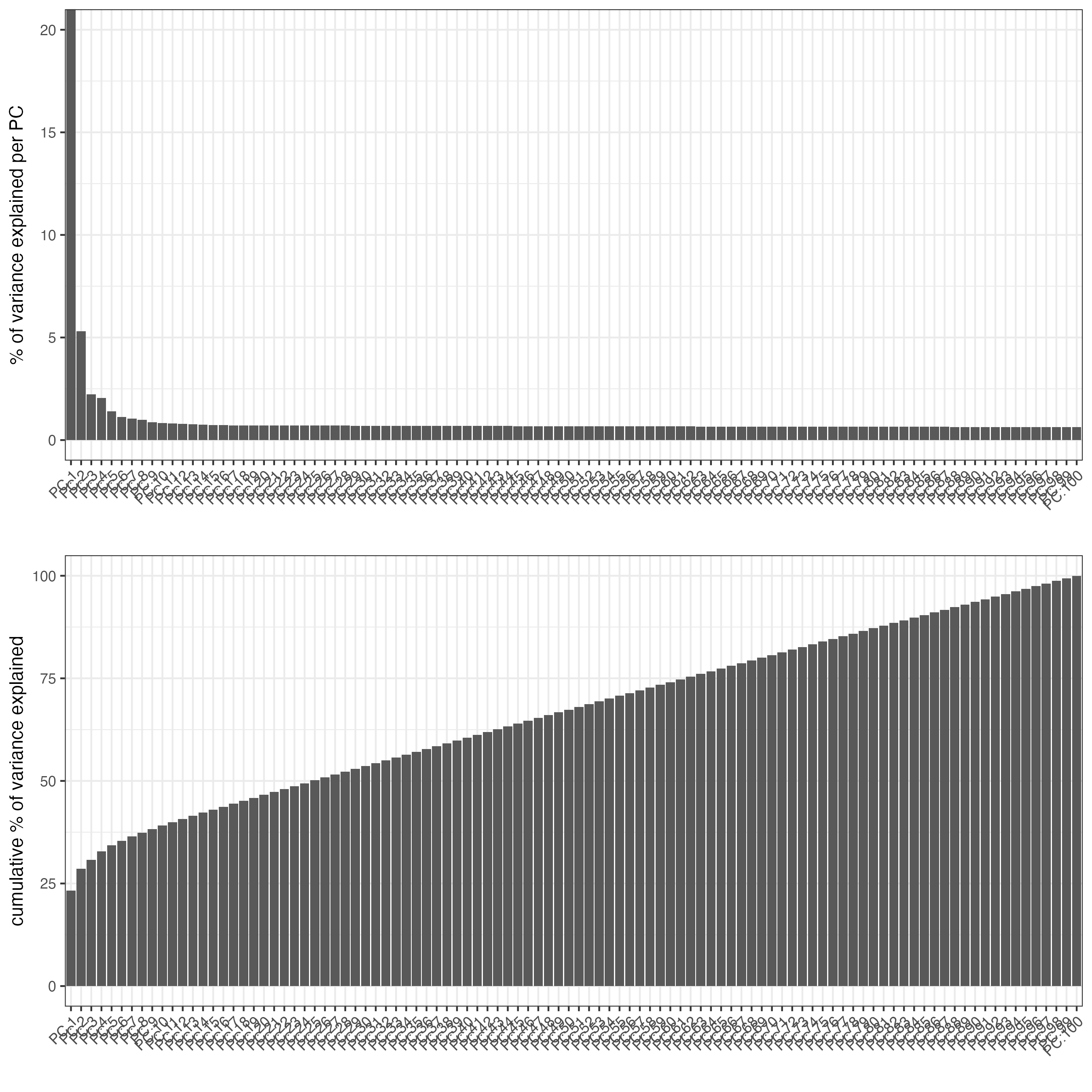
9.2 ATAC LSI
g <- runIterativeLSI(
    gobject = g,
    feat_type = "atac",
    expression_values = "raw",
    lsi_method = 2,
    resolution = 0.2,
    sample_cells_pre = 20000,
    var_features = 30000,
    dims = 30
)
10 Clustering
10.1 UMAP
# RNA
g <- runUMAP(g,
             feat_type = "rna")
# ATAC
g <- runUMAP(g,
             feat_type = "atac",
             dim_reduction_to_use = "lsi",
             dim_reduction_name = "atac_iterative_lsi")
10.2 Create shared nearest network (sNN) and perform Leiden clustering
# RNA
g <- createNearestNetwork(g,
                          feat_type = "rna")

g <- doLeidenCluster(g,
                     feat_type = "rna",
                     resolution = 0.8)

# ATAC
g <- createNearestNetwork(g,
                          feat_type = "atac",
                          dim_reduction_to_use = "lsi",
                          dim_reduction_name = "atac_iterative_lsi")

g <- doLeidenCluster(g,
                     feat_type = "atac",
                     network_name = "sNN.lsi",
                     resolution = 0.6,
                     name = "atac_leiden_clus")
10.3 Visualize UMAP cluster results
# RNA
plotUMAP(g,
         feat_type = "rna",
         cell_color = "leiden_clus",
         point_size = 3,
         cell_color_code = c("1" = "#FFDE7A",
                             "2" = "#FEFF05",
                             "3" = "#8BA0D1",
                             "4" = "#FF9C7A",
                             "5" = "#BFFF04",
                             "6" = "#FF8002",
                             "7" = "#01FFFF",
                             "8" = "#FF0000",
                             "9" = "#00BDBE",
                             "10" = "#C06BAA",
                             "11" = "#4000FF"
                             ),
         title = "RNA UMAP")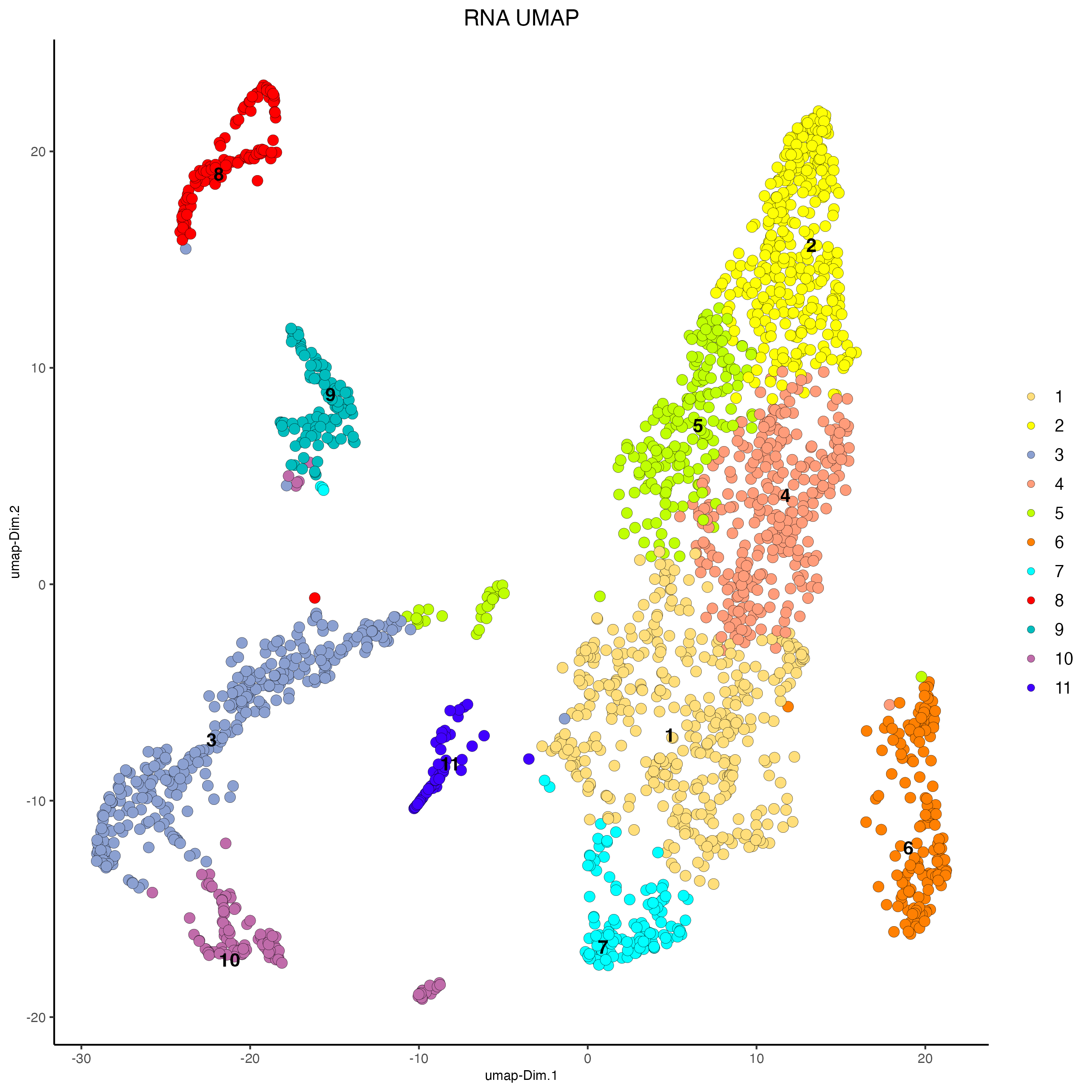
# ATAC
plotUMAP(g,
         feat_type = "atac",
         dim_reduction_name = "atac.umap",
         cell_color = "atac_leiden_clus",
         point_size = 3,
         cell_color_code = c("1" = "#8BA0D1",
                             "2" = "#FEFF05",
                             "3" = "#FF9C7A",
                             "4" = "#4a70f7",
                             "5" = "#FF0000",
                             "6" = "#FF8002",
                             "7" = "#C06BAA"
                             ),
         title = "ATAC UMAP")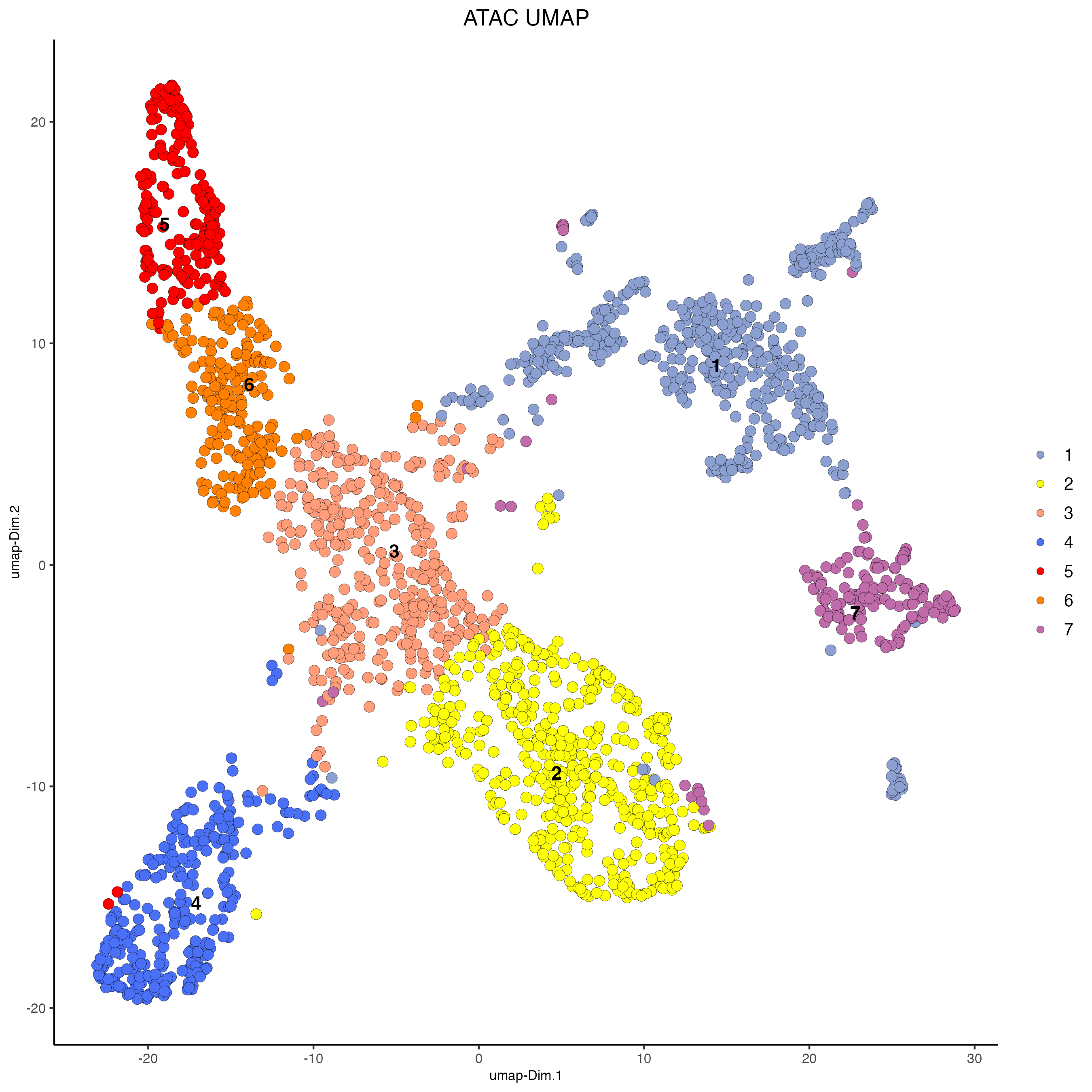
10.4 Visualize spatial results
# RNA
spatPlot2D(g,
           feat_type = "rna",
           cell_color = "leiden_clus",
           show_image = TRUE,
           point_size = 5,
           point_alpha = 0.5,
           cell_color_code = c("1" = "#FFDE7A",
                               "2" = "#FEFF05",
                               "3" = "#8BA0D1",
                               "4" = "#FF9C7A",
                               "5" = "#BFFF04",
                               "6" = "#FF8002",
                               "7" = "#01FFFF",
                               "8" = "#FF0000",
                               "9" = "#00BDBE",
                               "10" = "#C06BAA",
                               "11" = "#4000FF"
                               ),
           title = "RNA Leiden clusters")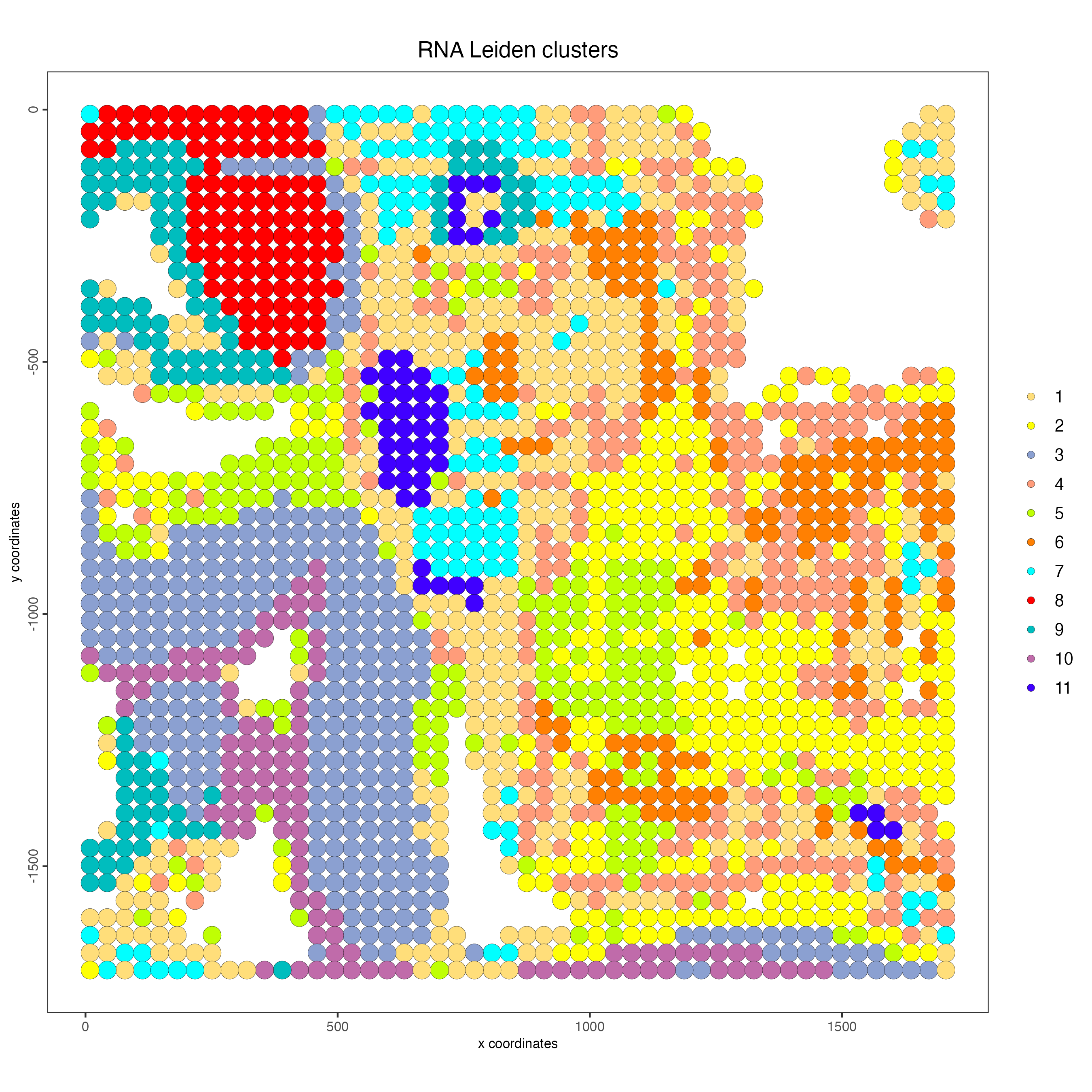
# ATAC
spatPlot2D(g,
           feat_type = "atac",
           cell_color = "atac_leiden_clus",
           point_size = 5,
           point_alpha = 0.5,
           show_image = TRUE,
           cell_color_code = c("1" = "#8BA0D1",
                               "2" = "#FEFF05",
                               "3" = "#FF9C7A",
                               "4" = "#4a70f7",
                               "5" = "#FF0000",
                               "6" = "#FF8002",
                               "7" = "#C06BAA"),
           title = "ATAC Leiden clusters")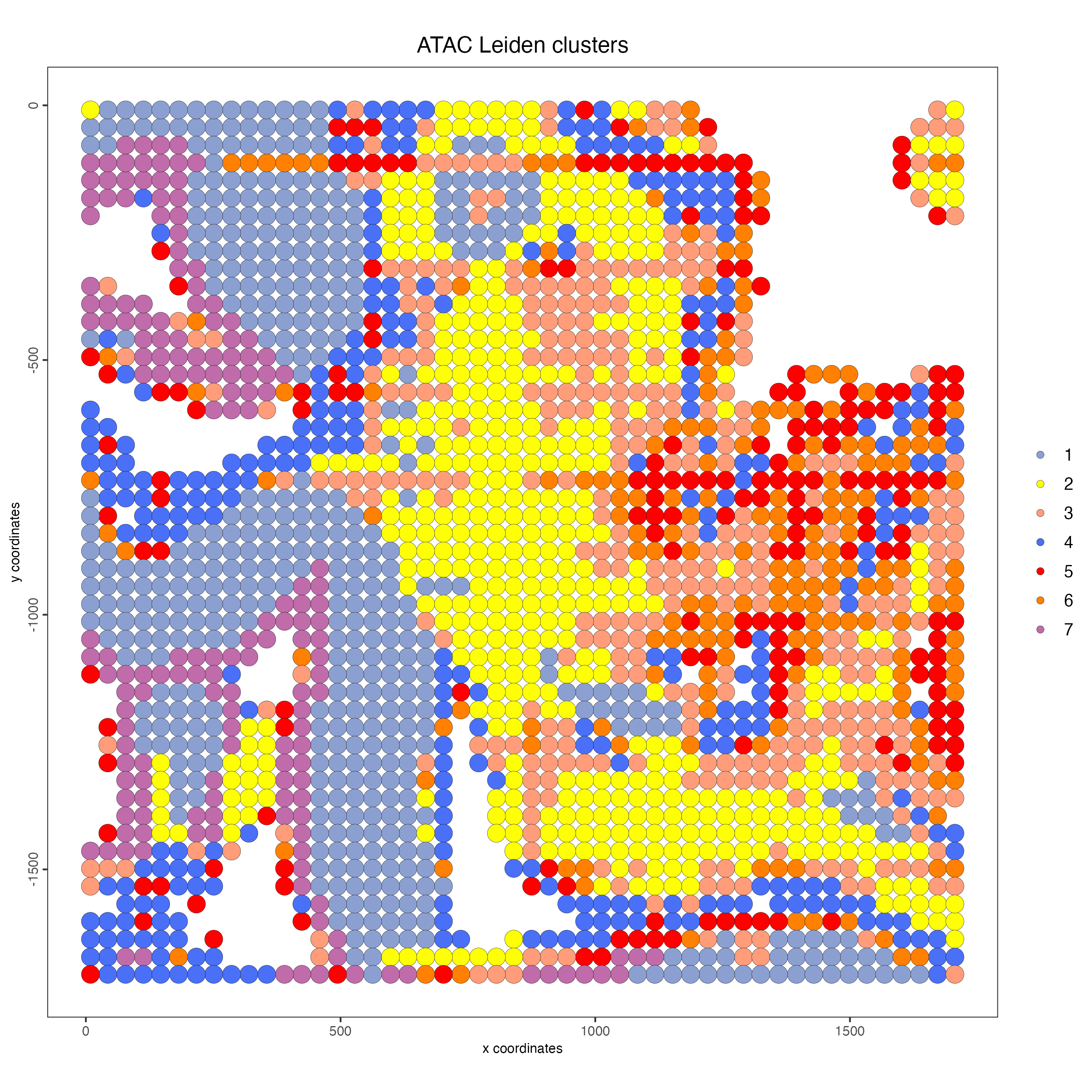
11 Multi-omics integration
11.1 Create k nearest network
# RNA
g <- createNearestNetwork(g,
                          feat_type = "rna",
                          type = "kNN",
                          dimensions_to_use = 1:10,
                          k = 10)

# ATAC
g <- createNearestNetwork(g,
                          feat_type = "atac",
                          dim_reduction_to_use = "lsi",
                          dim_reduction_name = "atac_iterative_lsi",
                          type = "kNN",
                          dimensions_to_use = 1:10,
k = 10)11.3 Create the integrated UMAP
g <- runIntegratedUMAP(
    gobject = g,
    spat_unit = "cell",
    feat_types = c("rna", "atac"),
    integrated_feat_type = "rna_atac",
    integration_method = "WNN",
    matrix_result_name = "theta_weighted_matrix",
    k = 10,
    spread = 10,
    min_dist = 0.01,
    force = TRUE,
    seed = 1234
)
11.4 Calculate integrated clusters
g <- doLeidenCluster(g,
                     feat_type = "rna",
                     nn_network_to_use = "kNN",
                     network_name = "integrated_kNN",
                     resolution = 1.2,
                     name = "integrated_leiden_clus")
11.5 Plot integrated UMAP
plotUMAP(g,
         feat_type = "rna",
         dim_reduction_name = "integrated.umap",
         cell_color = "integrated_leiden_clus",
         point_size = 3,
         cell_color_code = c("1" = "#BFFF04",
                             "2" = "#FEFF05",
                             "3" = "#FFDE7A",
                             "4" = "#FF00FF",
                             "5" = "#8BA0D1",
                             "6" = "#01FFFF",
                             "7" = "#4000FF",
                             "8" = "#FF8002",
                             "9" = "#FF0000",
                             "10" = "#f0b699",
                             "11" = "#4a70f7",
                             "12" = "#f09567",
                             "13" = "green",
                             "14" = "#1F8A42",
                             "15" = "#00BDBE",
                             "16" = "#C06BAA",
                             "17" = "#FF9C7A"
         ),
         title = "Integrated UMAP")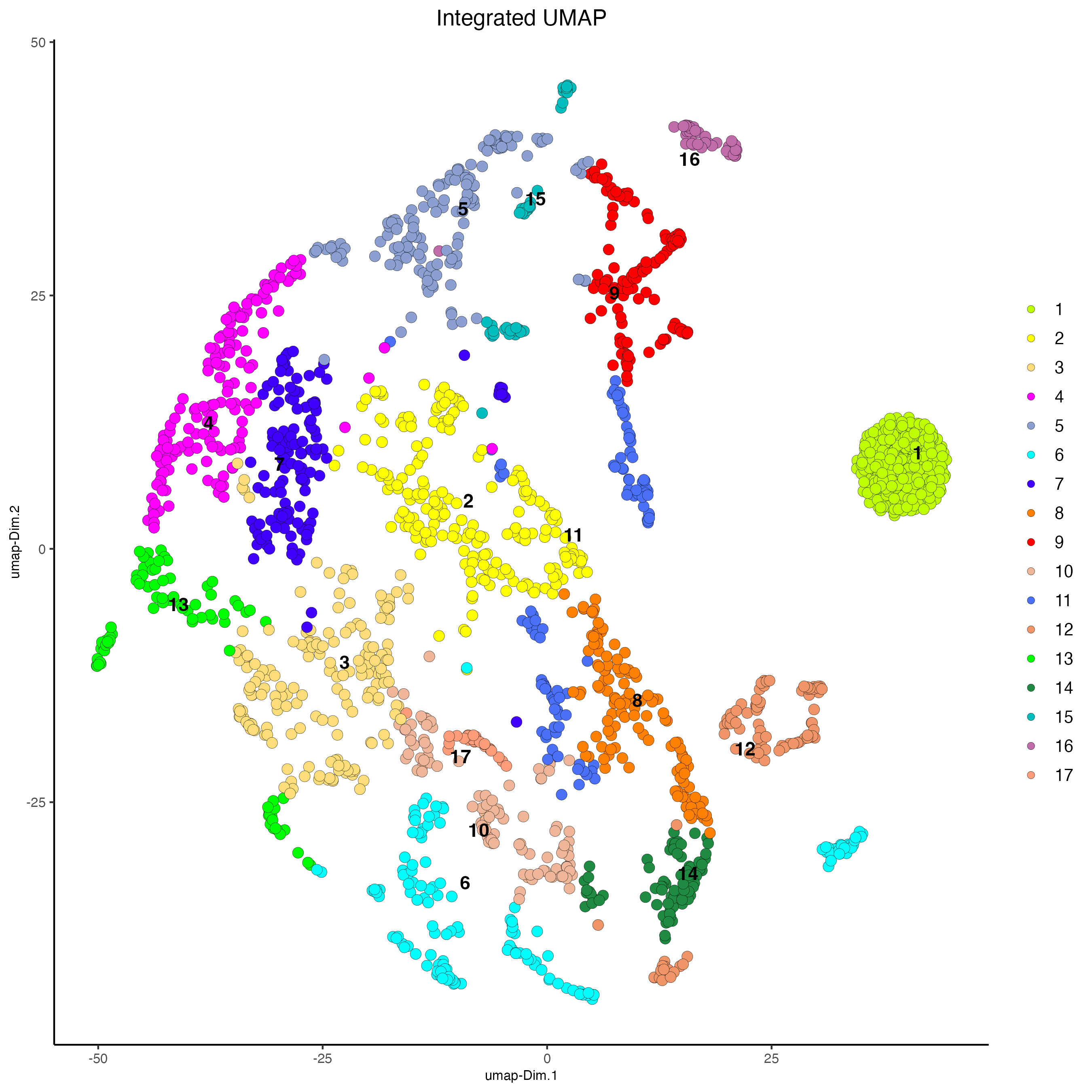
11.6 Plot spatial plot with integrated clusters
spatPlot2D(g,
           feat_type = "rna",
           cell_color = "integrated_leiden_clus",
           point_size = 5,
           cell_color_code = c("1" = "#BFFF04",
                               "2" = "#FEFF05",
                               "3" = "#FFDE7A",
                               "4" = "#FF00FF",
                               "5" = "#8BA0D1",
                               "6" = "#01FFFF",
                               "7" = "#4000FF",
                               "8" = "#FF8002",
                               "9" = "#FF0000",
                               "10" = "#f0b699",
                               "11" = "#4a70f7",
                               "12" = "#f09567",
                               "13" = "green",
                               "14" = "#1F8A42",
                               "15" = "#00BDBE",
                               "16" = "#C06BAA",
                               "17" = "#FF9C7A"
                               )
           ,
           title = "Integrated Leiden clusters")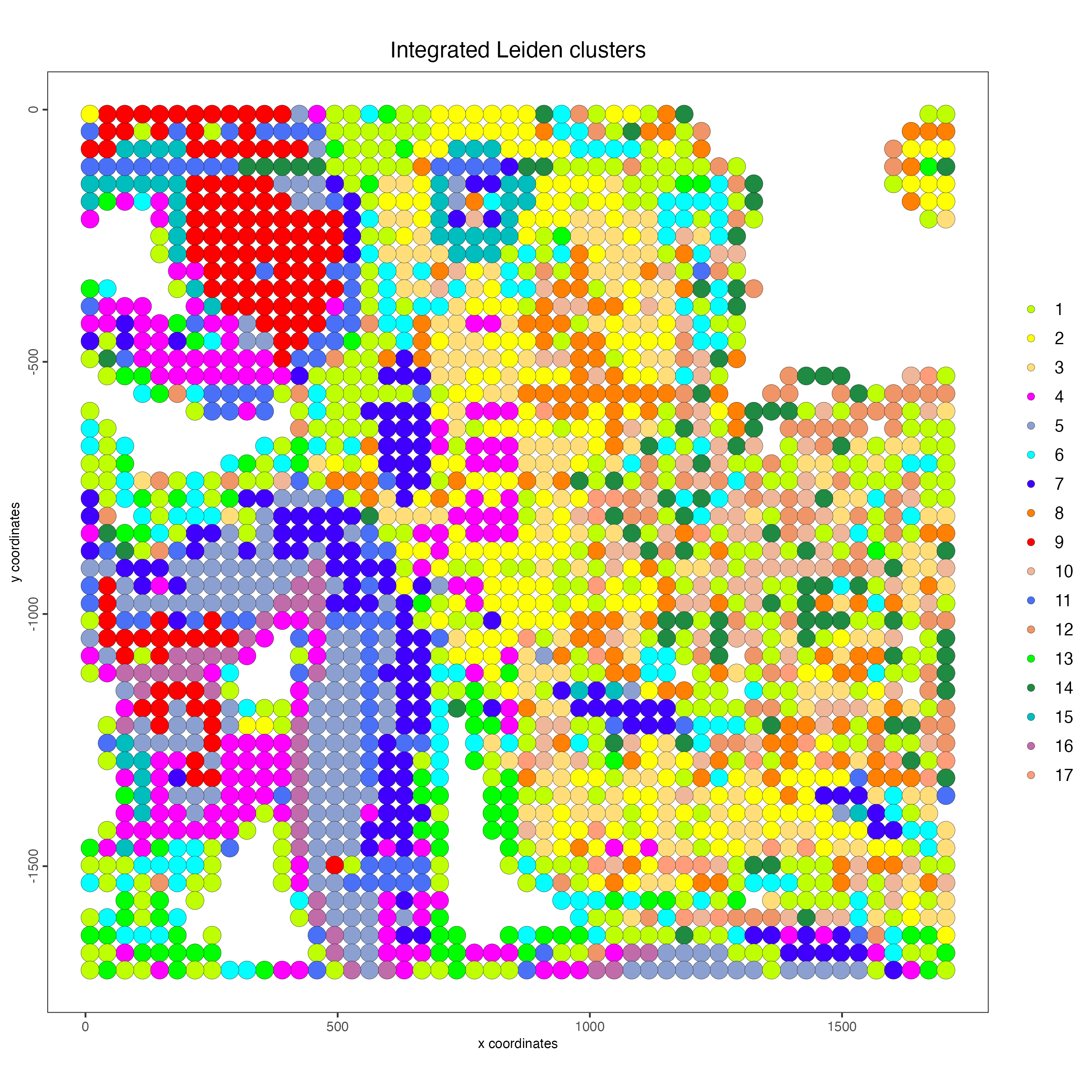
12 Session info
R version 4.4.2 (2024-10-31)
Platform: x86_64-apple-darwin20
Running under: macOS Sequoia 15.4.1

Matrix products: default
BLAS:   /System/Library/Frameworks/Accelerate.framework/Versions/A/Frameworks/vecLib.framework/Versions/A/libBLAS.dylib
LAPACK: /Library/Frameworks/R.framework/Versions/4.4-x86_64/Resources/lib/libRlapack.dylib;  LAPACK version 3.12.0

Random number generation:
 RNG:     L'Ecuyer-CMRG
 Normal:  Inversion
 Sample:  Rejection

locale:
[1] en_US.UTF-8/en_US.UTF-8/en_US.UTF-8/C/en_US.UTF-8/en_US.UTF-8

time zone: America/New_York
tzcode source: internal

attached base packages:
[1] stats4    grid      stats     graphics  grDevices utils     datasets  methods   base

other attached packages:
 [1] Giotto_4.2.1                GiottoClass_0.4.7           rhdf5_2.50.2
 [4] SummarizedExperiment_1.36.0 Biobase_2.66.0              RcppArmadillo_14.4.2-1
 [7] Rcpp_1.0.14                 Matrix_1.7-3                GenomicRanges_1.58.0
[10] GenomeInfoDb_1.42.3         IRanges_2.40.1              S4Vectors_0.44.0
[13] BiocGenerics_0.52.0         sparseMatrixStats_1.18.0    MatrixGenerics_1.18.1
[16] matrixStats_1.5.0           data.table_1.17.0           stringr_1.5.1
[19] plyr_1.8.9                  magrittr_2.0.3              ggplot2_3.5.2
[22] gtable_0.3.6                gtools_3.9.5                gridExtra_2.3
[25] devtools_2.4.5              usethis_3.1.0               ArchR_1.0.3

loaded via a namespace (and not attached):
  [1] RColorBrewer_1.1-3                 rstudioapi_0.17.1
  [3] jsonlite_2.0.0                     magick_2.8.6
  [5] farver_2.1.2                       ragg_1.4.0
  [7] fs_1.6.6                           BiocIO_1.16.0
  [9] zlibbioc_1.52.0                    vctrs_0.6.5
 [11] memoise_2.0.1                      Cairo_1.6-2
 [13] Rsamtools_2.22.0                   GiottoUtils_0.2.4
 [15] RCurl_1.98-1.17                    terra_1.8-42
 [17] htmltools_0.5.8.1                  S4Arrays_1.6.0
 [19] curl_6.2.2                         Rhdf5lib_1.28.0
 [21] SparseArray_1.6.2                  htmlwidgets_1.6.4
 [23] plotly_4.10.4                      cachem_1.1.0
 [25] GenomicAlignments_1.42.0           igraph_2.1.4
 [27] mime_0.13                          lifecycle_1.0.4
 [29] pkgconfig_2.0.3                    rsvd_1.0.5
 [31] R6_2.6.1                           fastmap_1.2.0
 [33] GenomeInfoDbData_1.2.13            shiny_1.10.0
 [35] digest_0.6.37                      colorspace_2.1-1
 [37] rprojroot_2.0.4                    irlba_2.3.5.1
 [39] pkgload_1.4.0                      textshaping_1.0.0
 [41] beachmat_2.22.0                    labeling_0.4.3
 [43] httr_1.4.7                         polyclip_1.10-7
 [45] abind_1.4-8                        compiler_4.4.2
 [47] here_1.0.1                         remotes_2.5.0
 [49] withr_3.0.2                        backports_1.5.0
 [51] BiocParallel_1.40.0                viridis_0.6.5
 [53] pkgbuild_1.4.7                     R.utils_2.13.0
 [55] ggforce_0.4.2                      MASS_7.3-65
 [57] DelayedArray_0.32.0                sessioninfo_1.2.3
 [59] rjson_0.2.23                       GiottoVisuals_0.2.12
 [61] tools_4.4.2                        httpuv_1.6.16
 [63] R.oo_1.27.0                        glue_1.8.0
 [65] dbscan_1.2.2                       restfulr_0.0.15
 [67] rhdf5filters_1.18.1                promises_1.3.2
 [69] checkmate_2.3.2                    generics_0.1.3
 [71] BSgenome_1.74.0                    R.methodsS3_1.8.2
 [73] tidyr_1.3.1                        ScaledMatrix_1.14.0
 [75] BiocSingular_1.22.0                tidygraph_1.3.1
 [77] XVector_0.46.0                     ggrepel_0.9.6
 [79] pillar_1.10.2                      later_1.4.2
 [81] dplyr_1.1.4                        tweenr_2.0.3
 [83] lattice_0.22-7                     FNN_1.1.4.1
 [85] rtracklayer_1.66.0                 tidyselect_1.2.1
 [87] SingleCellExperiment_1.28.1        Biostrings_2.74.1
 [89] miniUI_0.1.2                       scattermore_1.2
 [91] graphlayouts_1.2.2                 stringi_1.8.7
 [93] UCSC.utils_1.2.0                   lazyeval_0.2.2
 [95] yaml_2.3.10                        codetools_0.2-20
 [97] BSgenome.Mmusculus.UCSC.mm10_1.4.3 ggraph_2.2.1
 [99] tibble_3.2.1                       colorRamp2_0.1.0
[101] cli_3.6.5                          uwot_0.2.3
[103] systemfonts_1.2.2                  xtable_1.8-4
[105] reticulate_1.42.0                  dichromat_2.0-0.1
[107] png_0.1-8                          XML_3.99-0.18
[109] parallel_4.4.2                     ellipsis_0.3.2
[111] profvis_0.4.0                      urlchecker_1.0.1
[113] bitops_1.0-9                       SpatialExperiment_1.16.0
[115] viridisLite_0.4.2                  scales_1.4.0
[117] purrr_1.0.4                        crayon_1.5.3
[119] rlang_1.1.6                        cowplot_1.1.3