VisiumHD Human Colorectal Cancer
Source:vignettes/VisiumHD_Human_Colorectal_Cancer.Rmd
VisiumHD_Human_Colorectal_Cancer.Rmd1 Setup Giotto Environment
Ensure that the Giotto Suite is correctly installed and configured.
# Verify that the Giotto Suite is installed.
if(!"Giotto" %in% installed.packages()) {
  pak::pkg_install("drieslab/Giotto")
}

# check if the Python environment for Giotto has been installed.
genv_exists <- Giotto::checkGiottoEnvironment()
if(!genv_exists){
  # The following command need only be run once to install the Giotto environment.
  Giotto::installGiottoEnvironment()
}
2 Giotto global instructions and preparations
Set up the working directory and optionally specify a custom Python executable path if not using the default Giotto environment.
library(Giotto)

# 1. set working directory
results_folder <- "/path/to/results/"

python_path <- NULL # alternatively, "/local/python/path/python" if desired.
Create instructions for Giotto analysis, specifying the saving directory, whether to save plots, and the Python executable path if needed.
## create instructions
instructions <- createGiottoInstructions(
    save_dir = results_folder,
    save_plot = TRUE,
    show_plot = FALSE,
    return_plot = FALSE,
    python_path = python_path
)

## provide path to visium folder
data_path <- "/path/to/data/"
3 Download the dataset
options("timeout" = Inf)

download.file(
    url = "https://zenodo.org/records/13226158/files/workshop_VisiumHD.zip?download=1",
    destfile = file.path(data_path, "workshop_visiumHD.zip")
)

untar(
    tarfile = file.path(data_path, "workshop_visiumHD.zip"),
    exdir = data_path
)
4 Create Giotto object & process data
To create a Giotto object, you can either use visiumHD reader
function importVisiumHD() or read the data manually.
4.1 Using the reader function
readerHD <- importVisiumHD()

readerHD$visiumHD_dir <- file.path(data_path, "Human_Colorectal_Cancer_workshop/square_002um")

## directly from Visium folder
visiumHD <- readerHD$create_gobject(
    png_name = "tissue_lowres_image.png",
    gene_column_index = 2
)

## check metadata
pDataDT(visiumHD,
    spat_unit = "hex40"
)

# check available image names
showGiottoImageNames(visiumHD) # "image" is the default name
4.2 Read in data manually
4.2.1 Raw expression data
expression_path <- file.path(
    data_path,
    "/Human_Colorectal_Cancer_workshop/square_002um/raw_feature_bc_matrix"
)

expr_results <- get10Xmatrix(
    path_to_data = expression_path,
    gene_column_index = 1
)
4.2.2 Tissue positions data
tissue_positions_path <- file.path(
    data_path,
    "/Human_Colorectal_Cancer_workshop/square_002um/spatial/tissue_positions.parquet"
)

tissue_positions <- data.table::as.data.table(arrow::read_parquet(tissue_positions_path))
4.2.3 Merge expression and 2 micron position data
# convert expression matrix to minimal data.frame or data.table object
matrix_tile_dt <- data.table::as.data.table(Matrix::summary(expr_results))
genes <- expr_results@Dimnames[[1]]
samples <- expr_results@Dimnames[[2]]
matrix_tile_dt[, gene := genes[i]]
matrix_tile_dt[, pixel := samples[j]]
# merge data.table matrix and spatial coordinates to create input for Giotto Polygons
expr_pos_data <- data.table::merge.data.table(matrix_tile_dt,
    tissue_positions,
    by.x = "pixel",
    by.y = "barcode"
)

expr_pos_data <- expr_pos_data[, .(pixel, pxl_row_in_fullres, pxl_col_in_fullres, gene, x)]
colnames(expr_pos_data) <- c("pixel", "x", "y", "gene", "count")
4.3 Create giotto points
The giottoPoints object represents the spatial expression information for each transcript:
- gene id
- count or UMI
- spatial pixel location (x, y)
giotto_points <- createGiottoPoints(x = expr_pos_data[, .(x, y, gene, pixel, count)])4.4 Create giotto polygons
The Visium HD data is organized in a grid format. We can aggregate the data into larger bins to reduce the resolution of the data. Giotto Suite can work with any type of polygon information and already provides ready-to-use options for binning data with squares, triangles, and hexagons. Here we will use a hexagon tesselation to aggregate the data into arbitrary bins.
# create giotto polygons, here we create hexagons
hexbin400 <- tessellate(
    extent = ext(giotto_points),
    shape = "hexagon",
    shape_size = 400,
    name = "hex400"
)

plot(hexbin400)
4.5 Combine Giotto points and polygons to create Giotto object
# gpoints provides spatial gene expression information
# gpolygons provides spatial unit information (here = hexagon tiles)
visiumHD <- createGiottoObjectSubcellular(
    gpoints = list("rna" = giotto_points),
    gpolygons = list("hex400" = hexbin400),
    instructions = instructions
)

# create spatial centroids for each spatial unit (hexagon)
visiumHD <- addSpatialCentroidLocations(
    gobject = visiumHD,
    poly_info = "hex400"
)
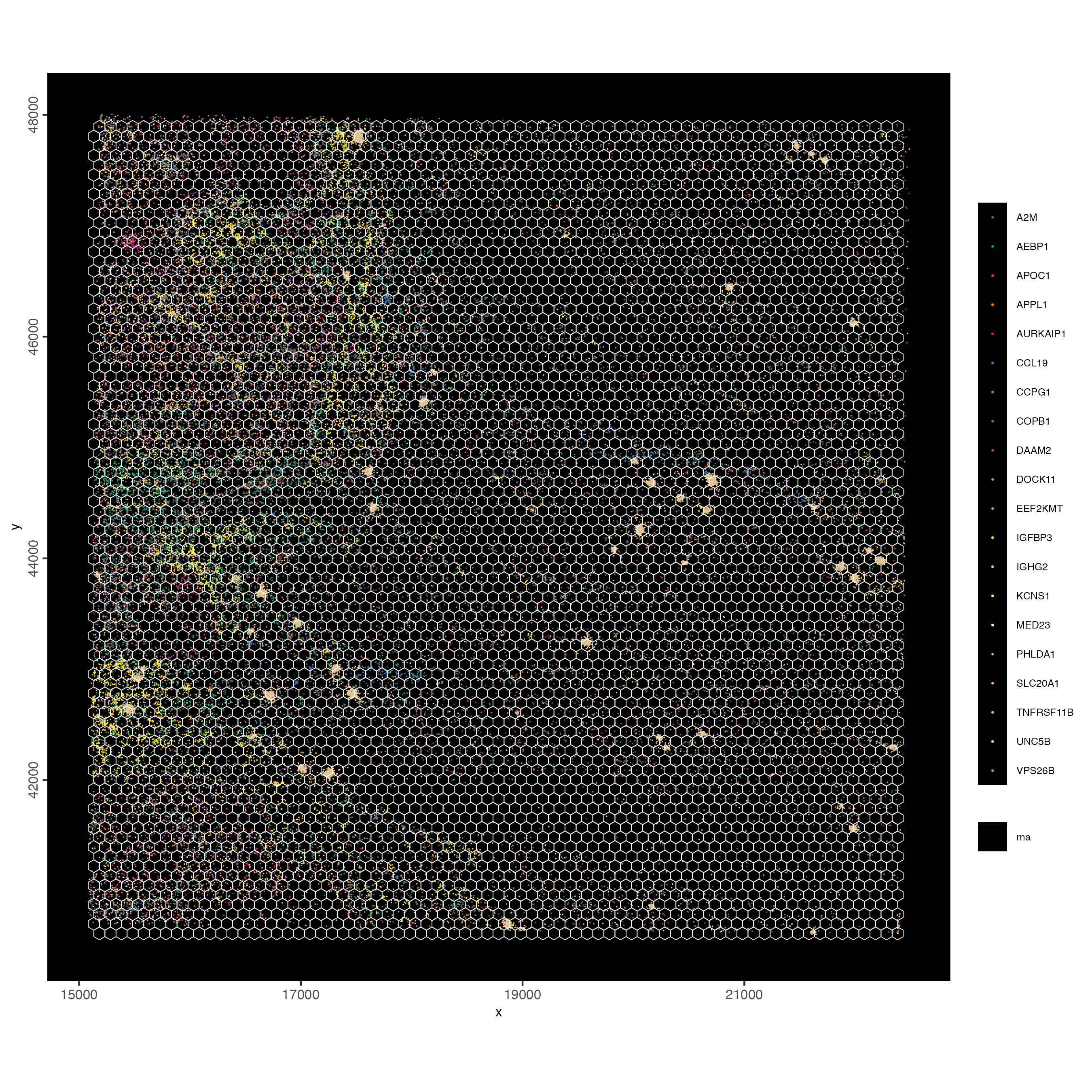
feature_data <- fDataDT(visiumHD)

spatInSituPlotPoints(visiumHD,
    show_image = FALSE,
    feats = list("rna" = feature_data$feat_ID[10:20]),
    show_legend = TRUE,
    spat_unit = "hex400",
    point_size = 0.25,
    show_polygon = TRUE,
    use_overlap = FALSE,
    polygon_feat_type = "hex400",
    polygon_bg_color = NA,
    polygon_color = "white",
    polygon_line_size = 0.1,
    expand_counts = TRUE,
    count_info_column = "count",
    jitter = c(25, 25)
)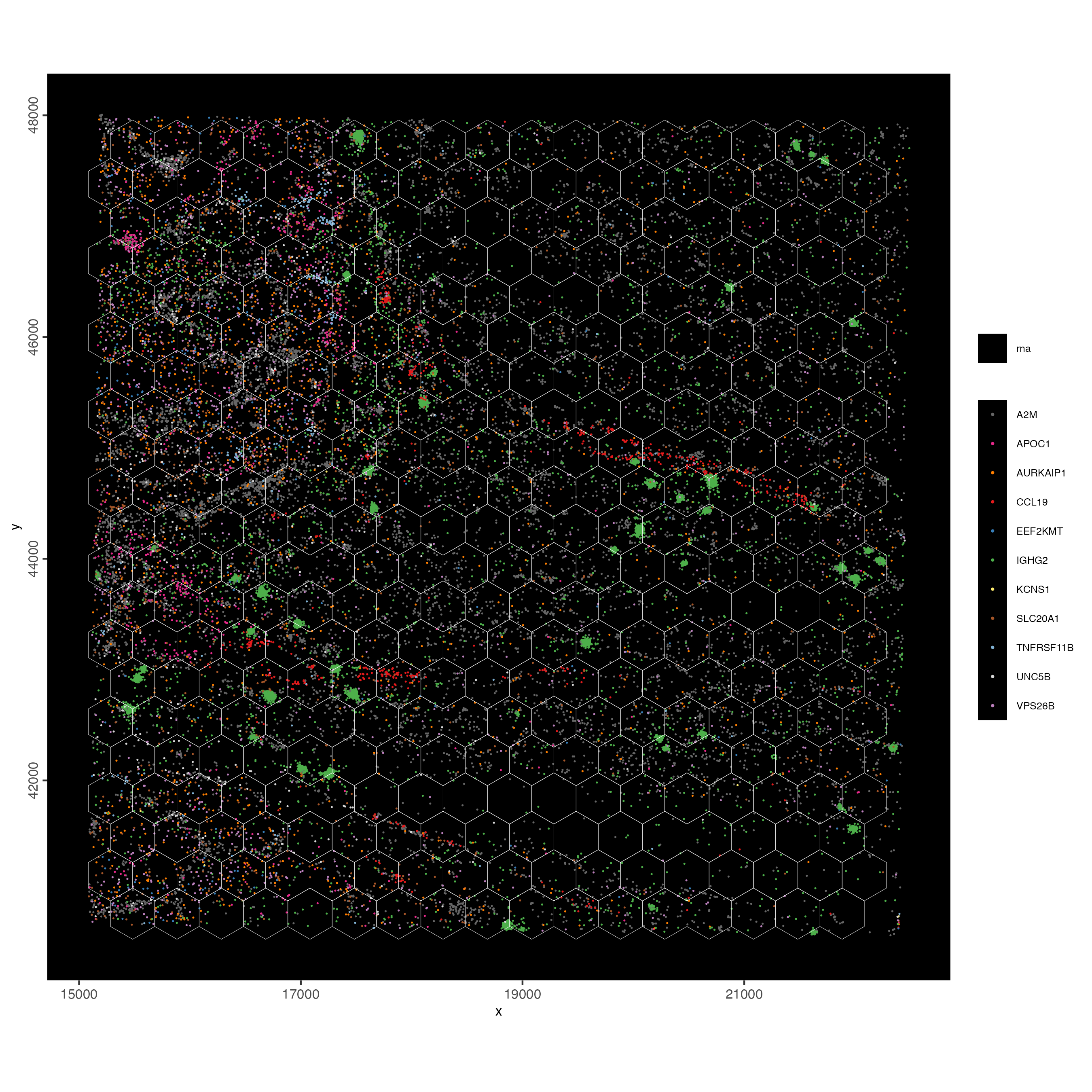
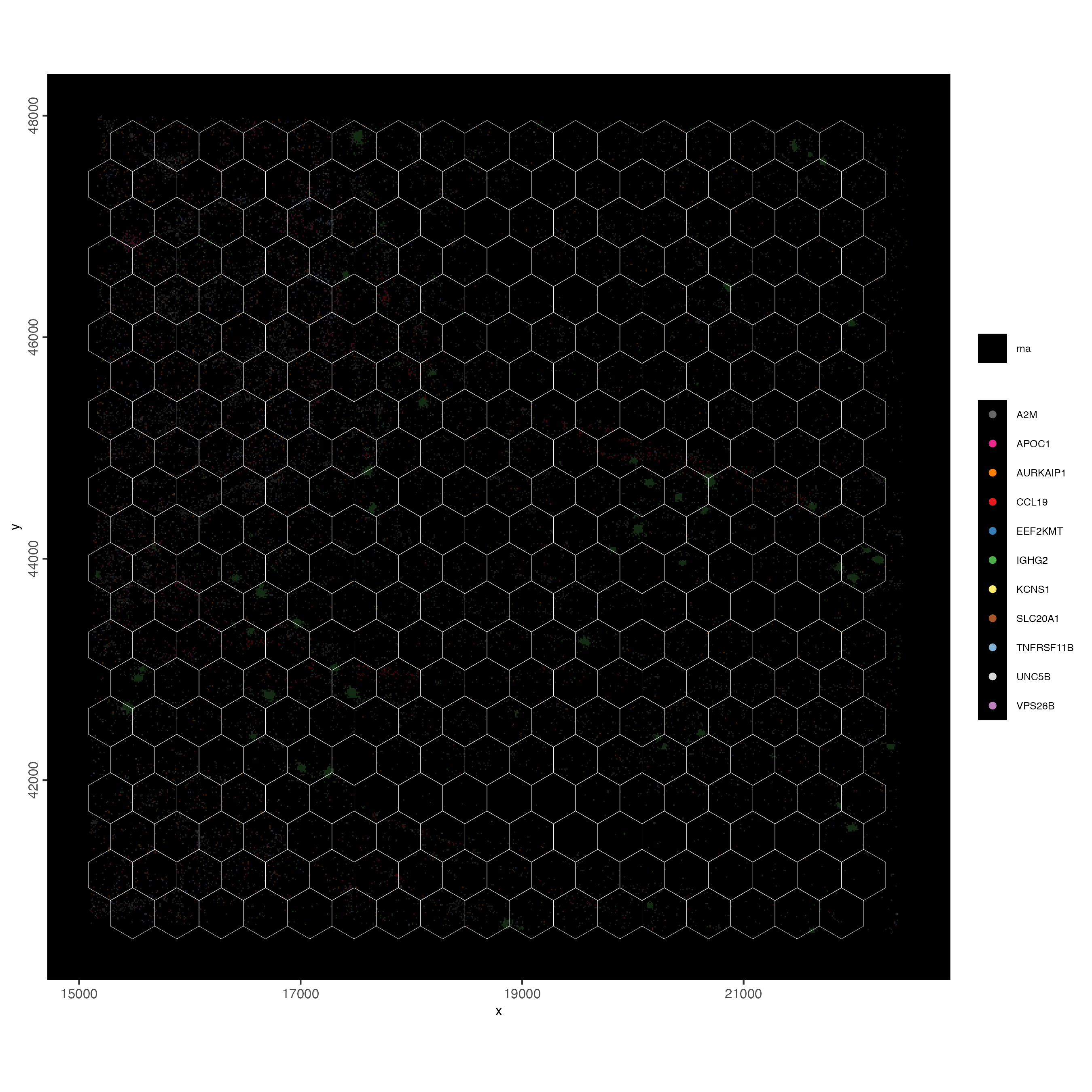
You can set plot_method = scattermore or scattermost to convert high-resolution images to low(er) resolution rasterized images. It’s usually faster and will save on disk space.
spatInSituPlotPoints(visiumHD,
    show_image = FALSE,
    feats = list("rna" = feature_data$feat_ID[10:20]),
    show_legend = TRUE,
    spat_unit = "hex400",
    point_size = 0.25,
    show_polygon = TRUE,
    use_overlap = FALSE,
    polygon_feat_type = "hex400",
    polygon_bg_color = NA,
    polygon_color = "white",
    polygon_line_size = 0.1,
    expand_counts = TRUE,
    count_info_column = "count",
    jitter = c(25, 25),
    plot_method = "scattermore"
)
5 Hexbin 400
5.1 Calculate overlap between points and polygons
At the moment the giotto points (transcripts) and polygons (hexagons) are two separate layers of information. Here we will determine which transcripts overlap with which hexagons so that we can aggregate the gene expression information and convert this into a gene expression matrix (genes-by-hexagons) that can be used in default spatial pipelines.
# calculate overlap between points and polygons
visiumHD <- calculateOverlap(visiumHD,
    spatial_info = "hex400",
    feat_info = "rna"
)

showGiottoSpatialInfo(visiumHD)
5.2 Convert overlap results to a gene-by-hexagon matrix
# convert overlap results to bin by gene matrix
visiumHD <- overlapToMatrix(visiumHD,
    poly_info = "hex400",
    feat_info = "rna",
    name = "raw"
)

# this action will automatically create an active spatial unit, e.g. hexbin 400
activeSpatUnit(visiumHD)
5.3 Default processing steps
Perform data processing including filtering, normalization, and adding optional statistics.
# filter on gene expression matrix
visiumHD <- filterGiotto(visiumHD,
expression_threshold = 1,
feat_det_in_min_cells = 5,
min_det_feats_per_cell = 25
)
# normalize and scale gene expression data
visiumHD <- normalizeGiotto(visiumHD,
scalefactor = 1000,
verbose = TRUE
)
# add cell and gene statistics
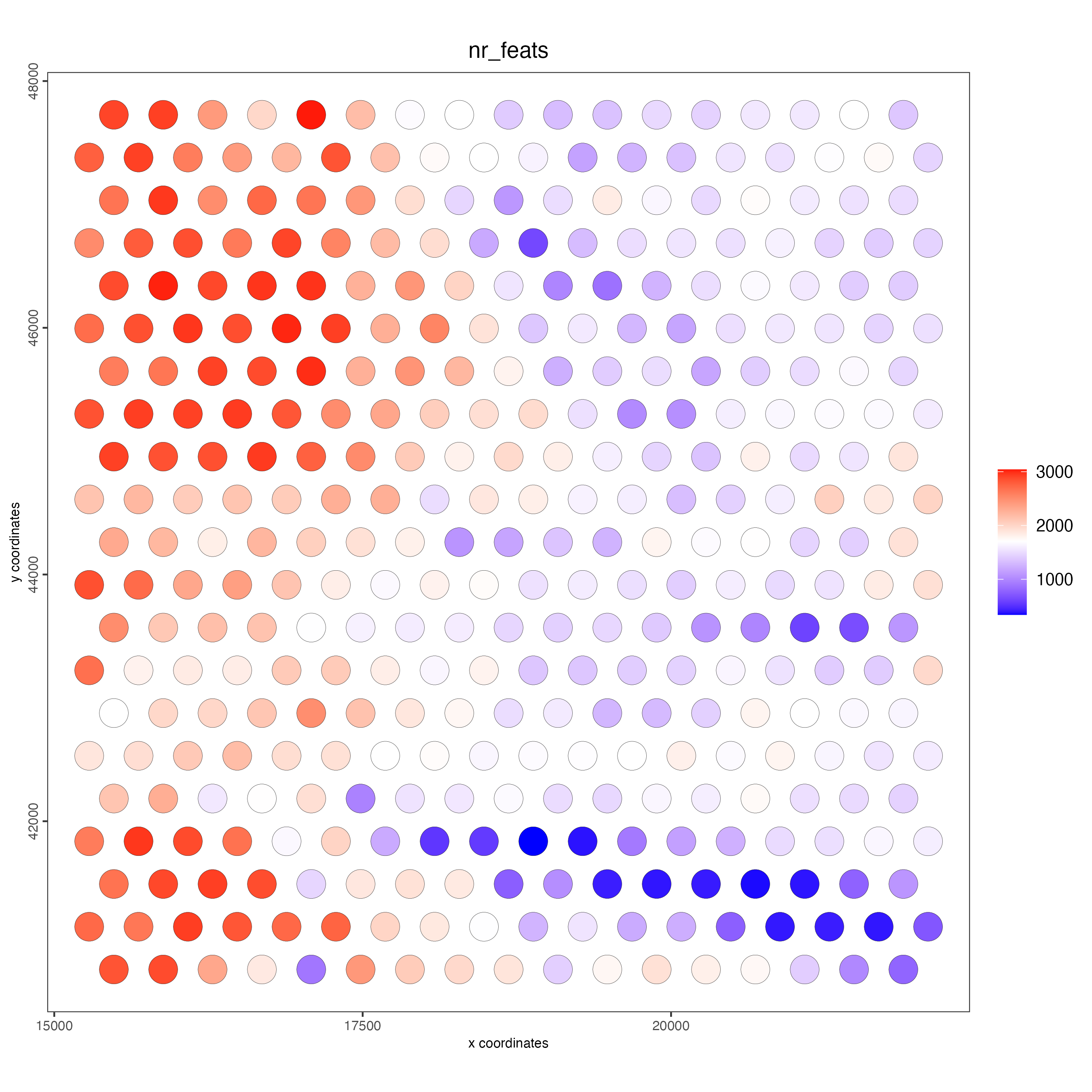
visiumHD <- addStatistics(visiumHD)5.4 Visualize the number of features
# each dot here represents a 200x200 aggregation of spatial barcodes (bin size 200)
spatPlot2D(
    gobject = visiumHD,
    cell_color = "nr_feats",
    color_as_factor = FALSE,
    point_size = 8
)
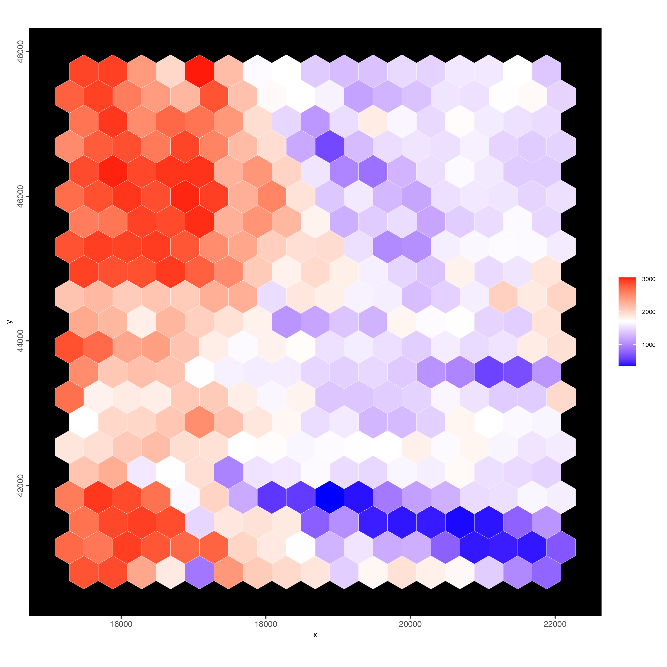
Using the spatial polygon (hexagon) tiles
spatInSituPlotPoints(visiumHD,
    show_image = FALSE,
    feats = NULL,
    show_legend = FALSE,
    spat_unit = "hex400",
    point_size = 0.1,
    show_polygon = TRUE,
    use_overlap = TRUE,
    polygon_feat_type = "hex400",
    polygon_fill = "nr_feats",
    polygon_fill_as_factor = FALSE,
    polygon_bg_color = NA,
    polygon_color = "white",
    polygon_line_size = 0.1
)
5.5 Dimension reduction
visiumHD <- calculateHVF(visiumHD,
zscore_threshold = 1
)
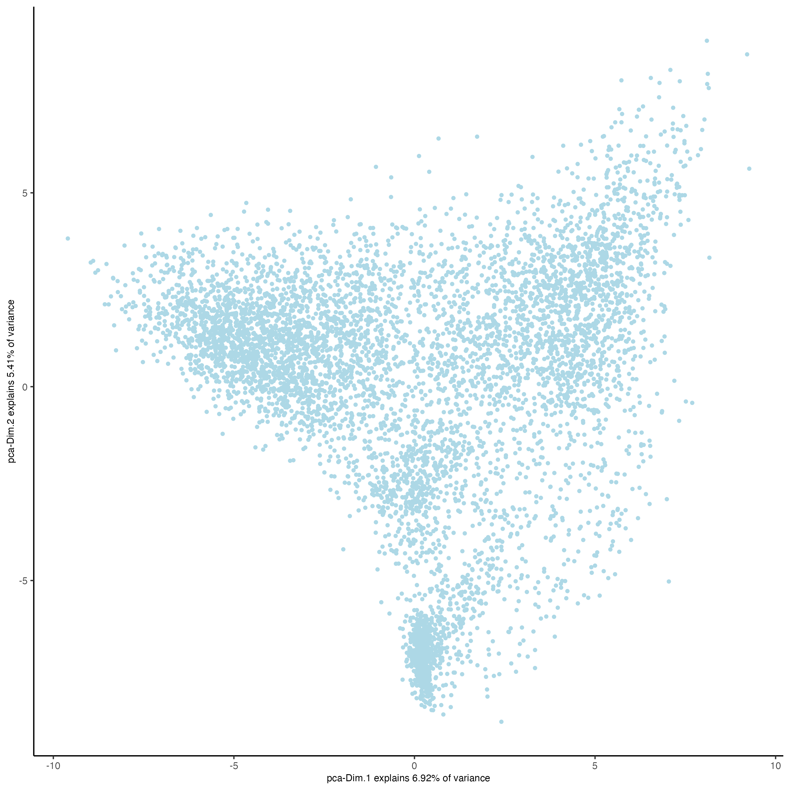
visiumHD <- runPCA(visiumHD,
expression_values = "normalized",
feats_to_use = "hvf"
)
screePlot(visiumHD, ncp = 30)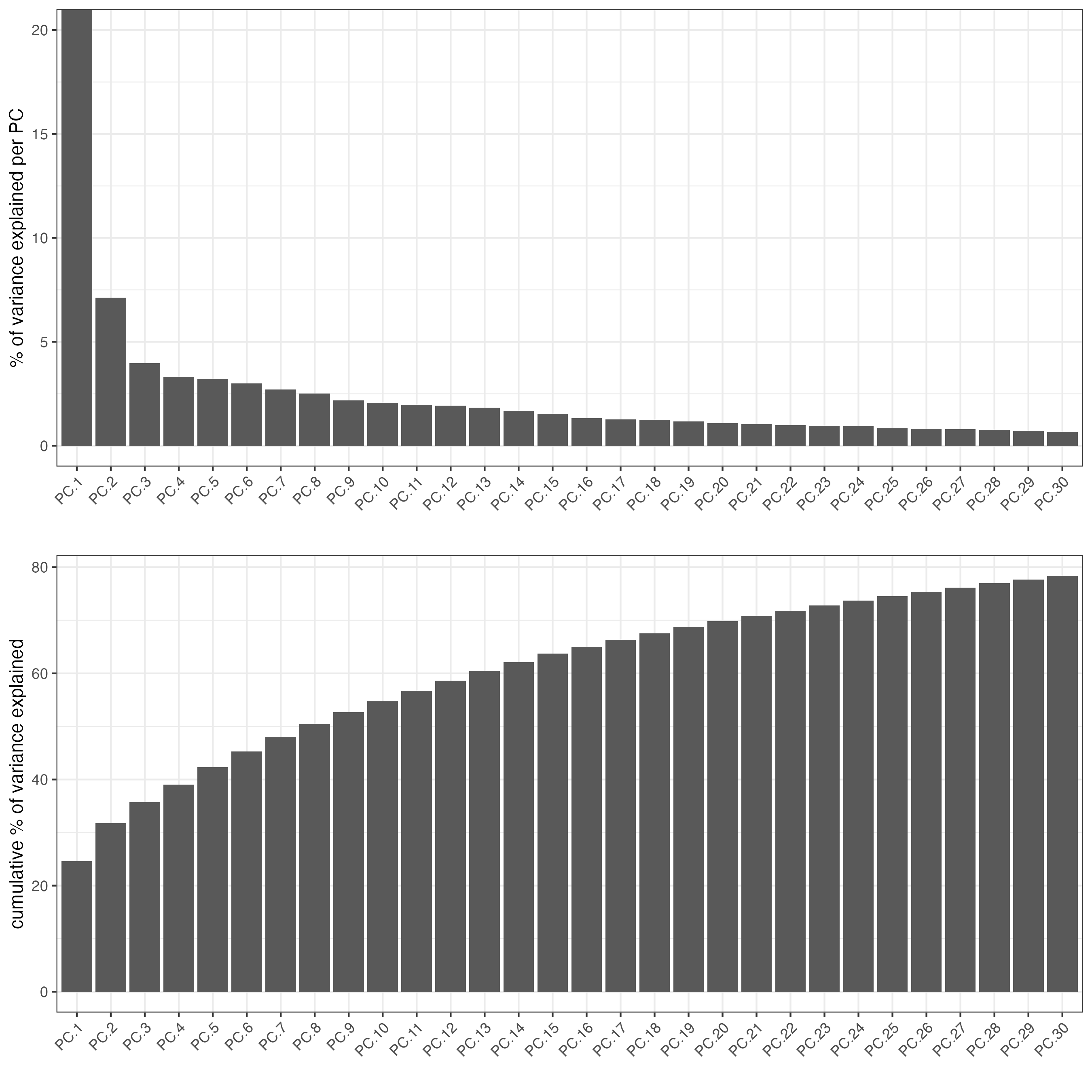
plotPCA(visiumHD)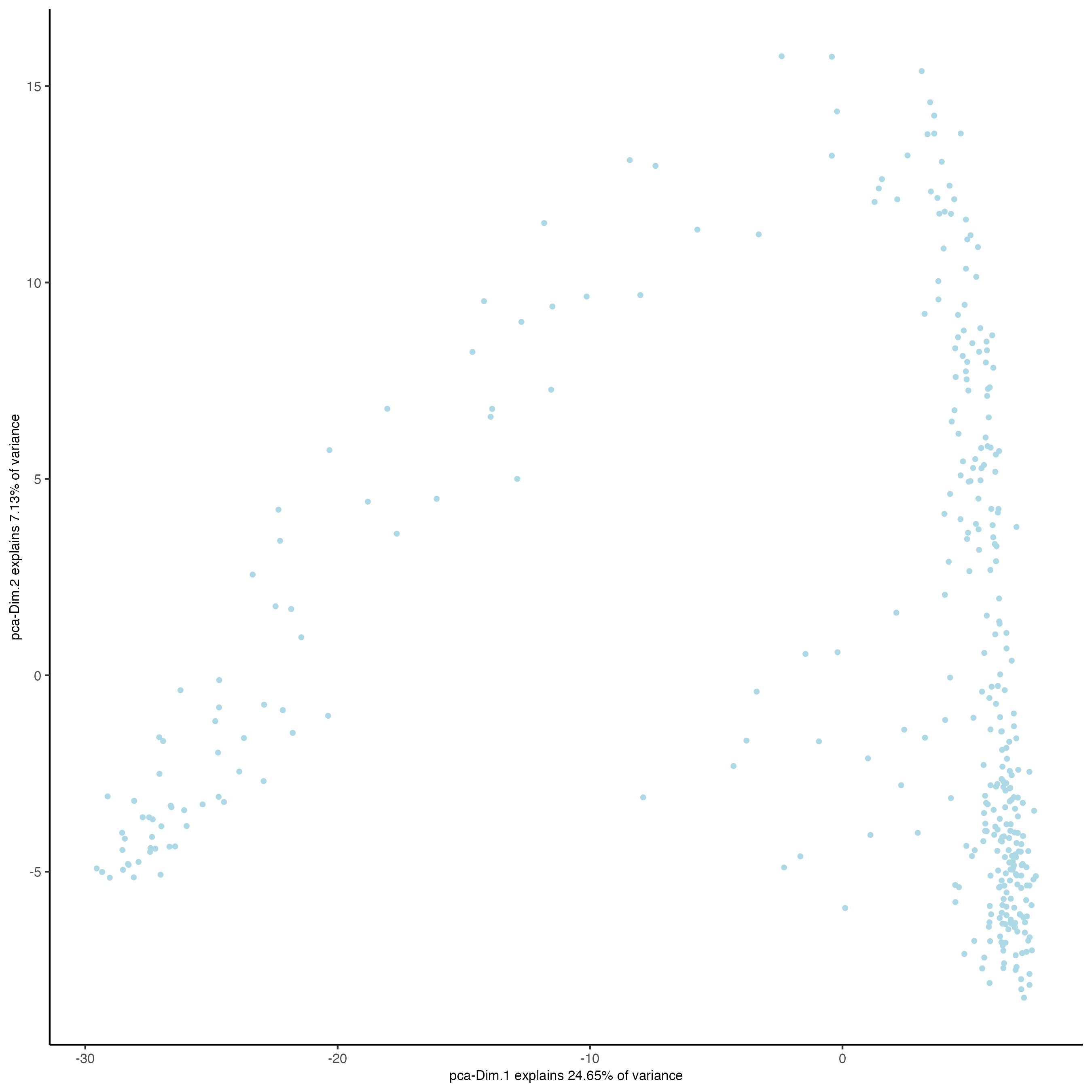
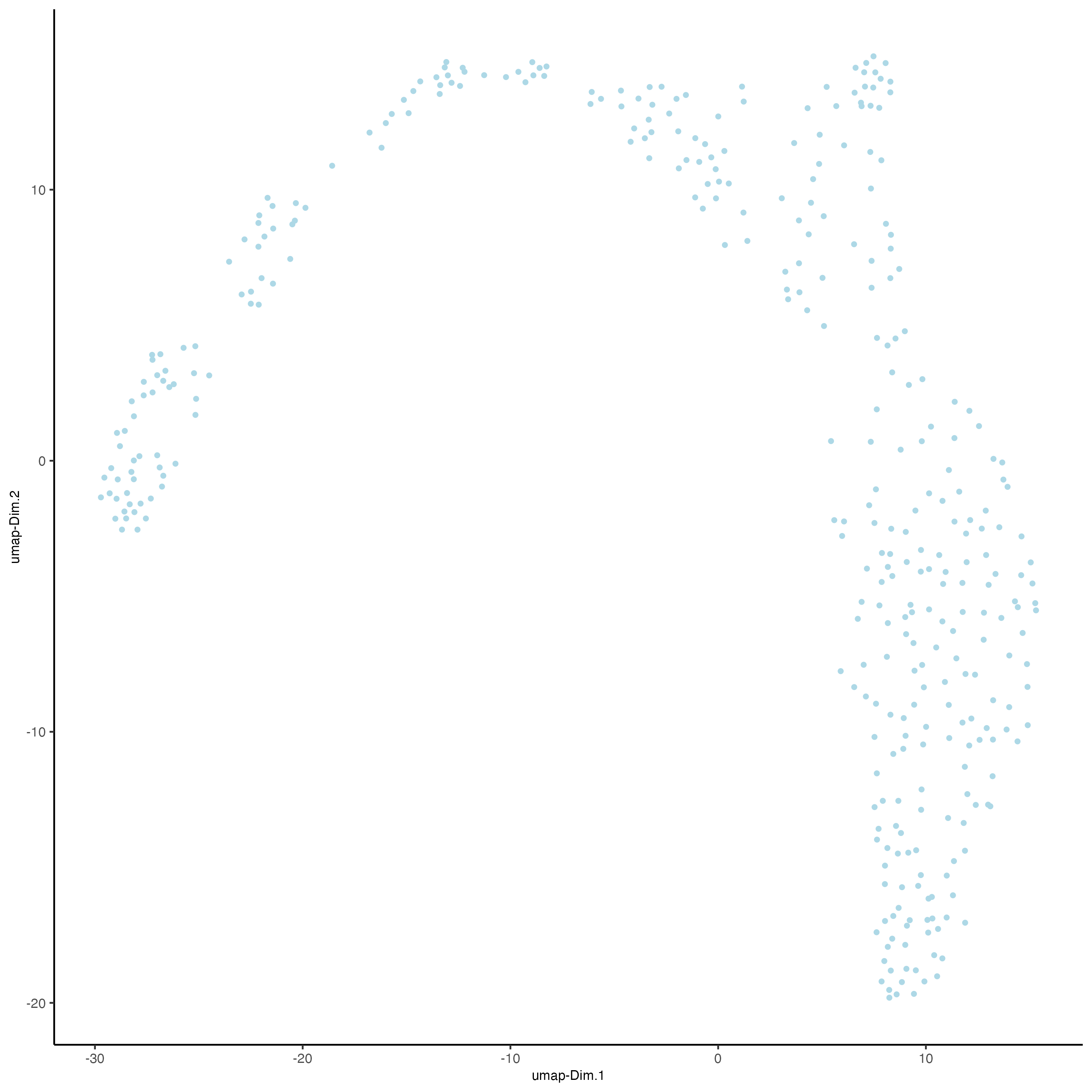
5.6 Clustering
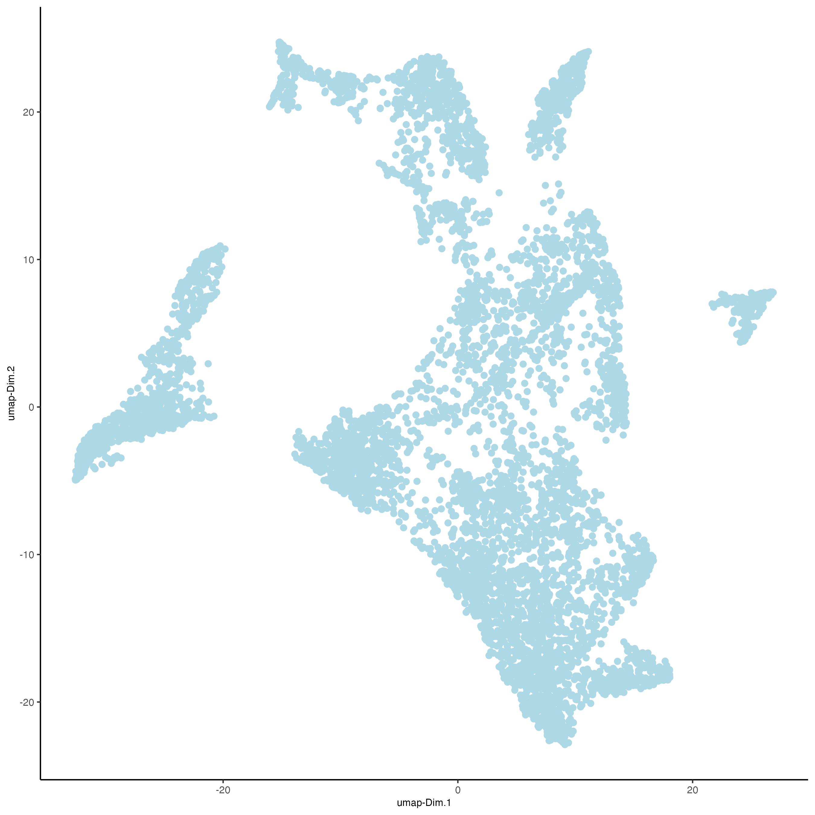
visiumHD <- runUMAP(visiumHD,
    dimensions_to_use = 1:14,
    n_threads = 10
)

plotUMAP(visiumHD,
    point_size = 1
)
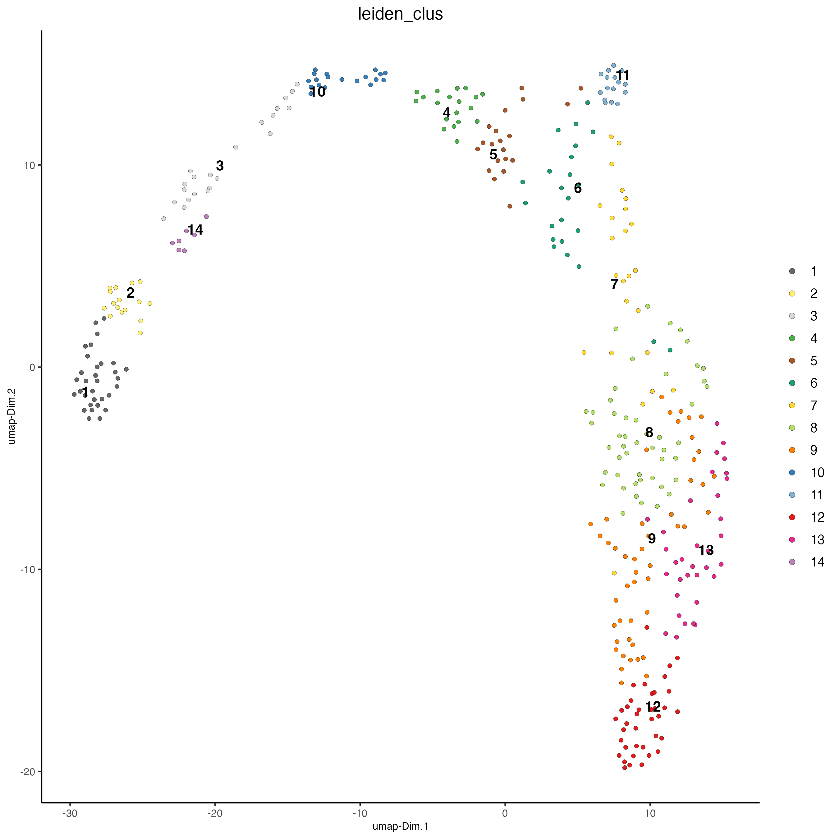
# sNN network (default)
visiumHD <- createNearestNetwork(visiumHD,
    dimensions_to_use = 1:14,
    k = 5
)

## Leiden clustering ####
visiumHD <- doLeidenClusterIgraph(visiumHD,
    resolution = 0.5,
    n_iterations = 1000,
    spat_unit = "hex400"
)
plotUMAP(
    gobject = visiumHD,
    cell_color = "leiden_clus",
    point_size = 1.5,
    show_NN_network = FALSE,
    edge_alpha = 0.05
)
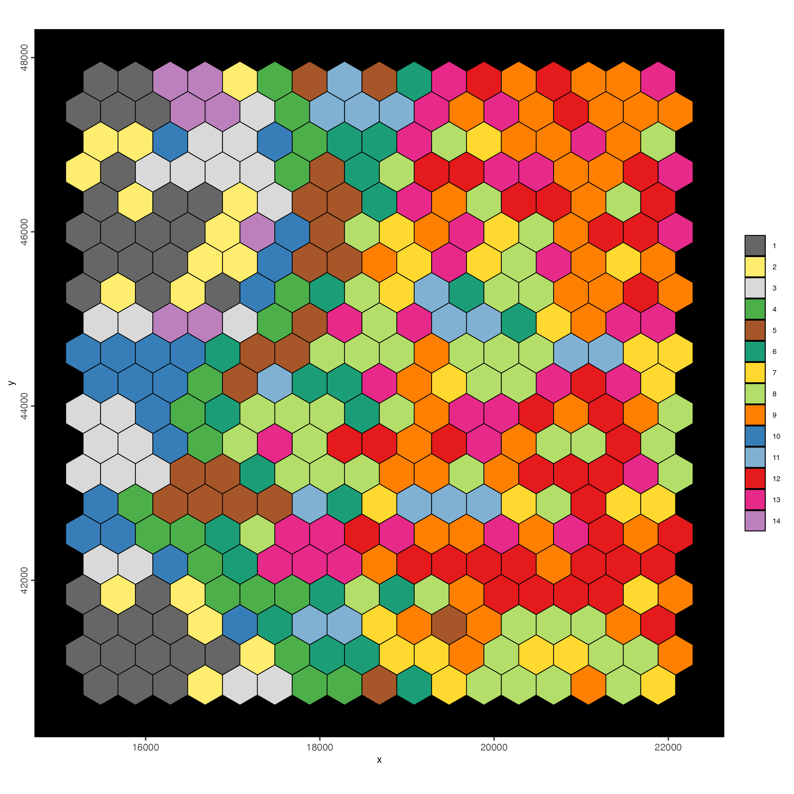
spatInSituPlotPoints(visiumHD,
    show_image = FALSE,
    feats = NULL,
    show_legend = FALSE,
    spat_unit = "hex400",
    point_size = 0.25,
    show_polygon = TRUE,
    use_overlap = FALSE,
    polygon_feat_type = "hex400",
    polygon_fill_as_factor = TRUE,
    polygon_fill = "leiden_clus",
    polygon_color = "black",
    polygon_line_size = 0.3
)
6 Hexbin 100
Observation: Hexbin 400 results in very coarse information about the tissue.
The goal is to create a higher resolution bin (hex100), then add this to the Giotto object to compare difference in resolution.
6.1 Standard subcellular pipeline
- Create new spatial unit layer, e.g. with tessellate function
- Add spatial units to Giottoo object
- Calculate centroids (optional)
- Compute overlap between transcript and polygon (hexagon) locations.
- Convert overlap data into a gene-by-polygon matrix
hexbin100 <- tessellate(
    extent = ext(visiumHD),
    shape = "hexagon",
    shape_size = 100,
    name = "hex100"
)

visiumHD <- setPolygonInfo(
    gobject = visiumHD,
    x = hexbin100,
    name = "hex100",
    initialize = TRUE
)

visiumHD <- addSpatialCentroidLocations(
    gobject = visiumHD,
    poly_info = "hex100"
)
Set active spatial unit. This can also be set manually in each function.
activeSpatUnit(visiumHD) <- "hex100"
spatInSituPlotPoints(visiumHD,
    show_image = FALSE,
    feats = list("rna" = feature_data$feat_ID[1:20]),
    show_legend = TRUE,
    spat_unit = "hex100",
    point_size = 0.1,
    show_polygon = TRUE,
    use_overlap = FALSE,
    polygon_feat_type = "hex100",
    polygon_bg_color = NA,
    polygon_color = "white",
    polygon_line_size = 0.2,
    expand_counts = TRUE,
    count_info_column = "count",
    jitter = c(25, 25)
)
visiumHD <- calculateOverlap(visiumHD,
    spatial_info = "hex100",
    feat_info = "rna"
)

visiumHD <- overlapToMatrix(visiumHD,
    poly_info = "hex100",
    feat_info = "rna",
    name = "raw"
)

visiumHD <- filterGiotto(visiumHD,
    spat_unit = "hex100",
    expression_threshold = 1,
    feat_det_in_min_cells = 10,
    min_det_feats_per_cell = 10
)

visiumHD <- normalizeGiotto(visiumHD,
    spat_unit = "hex100",
    scalefactor = 1000,
    verbose = TRUE
)

visiumHD <- addStatistics(visiumHD,
    spat_unit = "hex100"
)
Your Giotto object will have metadata for each spatial unit.
visiumHD <- calculateHVF(visiumHD,
    spat_unit = "hex100",
    zscore_threshold = 1
)

visiumHD <- runPCA(visiumHD,
    spat_unit = "hex100",
    expression_values = "normalized",
    feats_to_use = "hvf"
)

plotPCA(visiumHD,
    spat_unit = "hex100"
)
visiumHD <- runUMAP(visiumHD,
    spat_unit = "hex100",
    dimensions_to_use = 1:14,
    n_threads = 10
)

# plot UMAP, coloring cells/points based on nr_feats
plotUMAP(
    gobject = visiumHD,
    spat_unit = "hex100",
    point_size = 2
)
# sNN network (default)
visiumHD <- createNearestNetwork(visiumHD,
spat_unit = "hex100",
dimensions_to_use = 1:14,
k = 5
)
## leiden clustering ####
visiumHD <- doLeidenClusterIgraph(visiumHD,
spat_unit = "hex100",
resolution = 0.2,
n_iterations = 1000
)
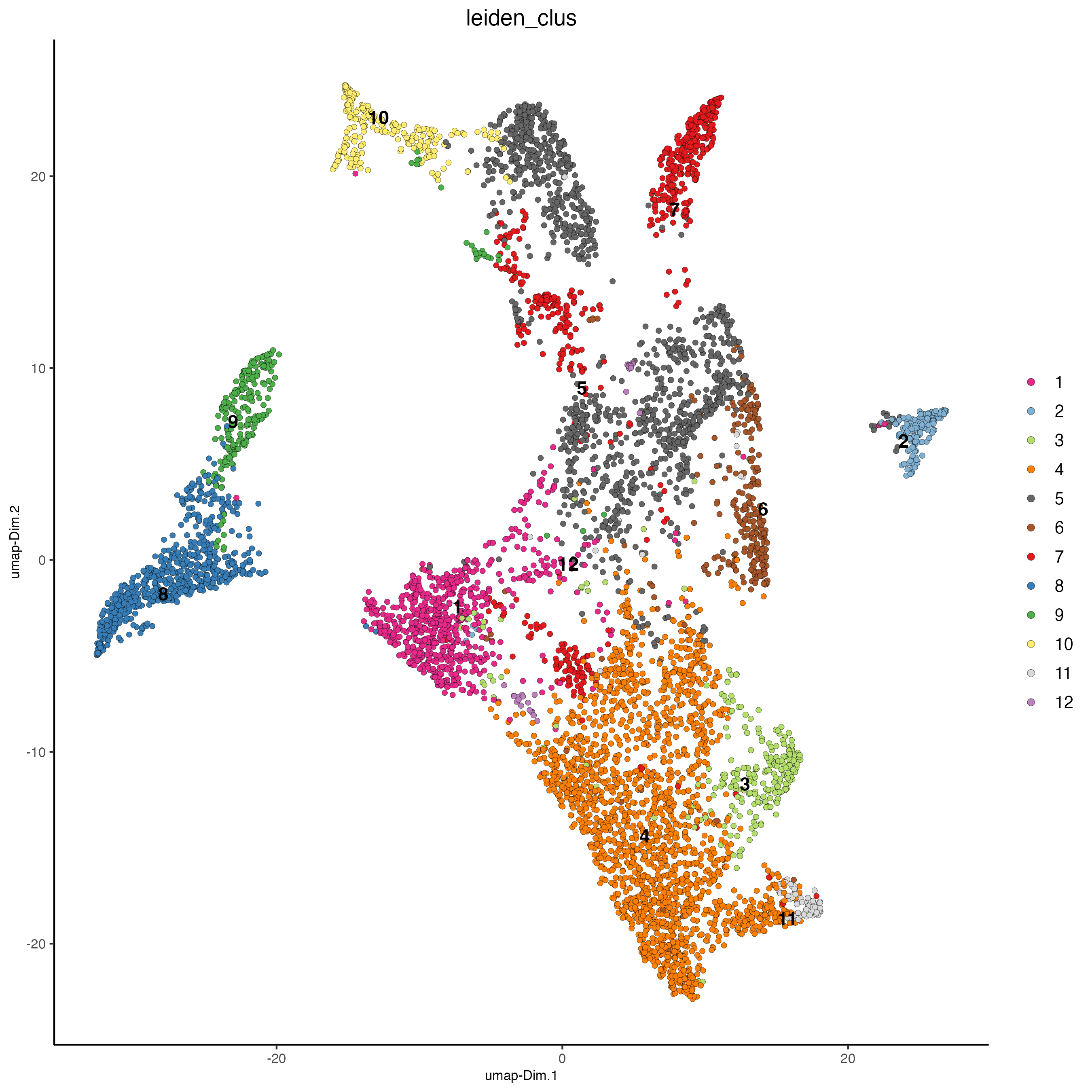
plotUMAP(
gobject = visiumHD,
spat_unit = "hex100",
cell_color = "leiden_clus",
point_size = 1.5,
show_NN_network = FALSE,
edge_alpha = 0.05
)
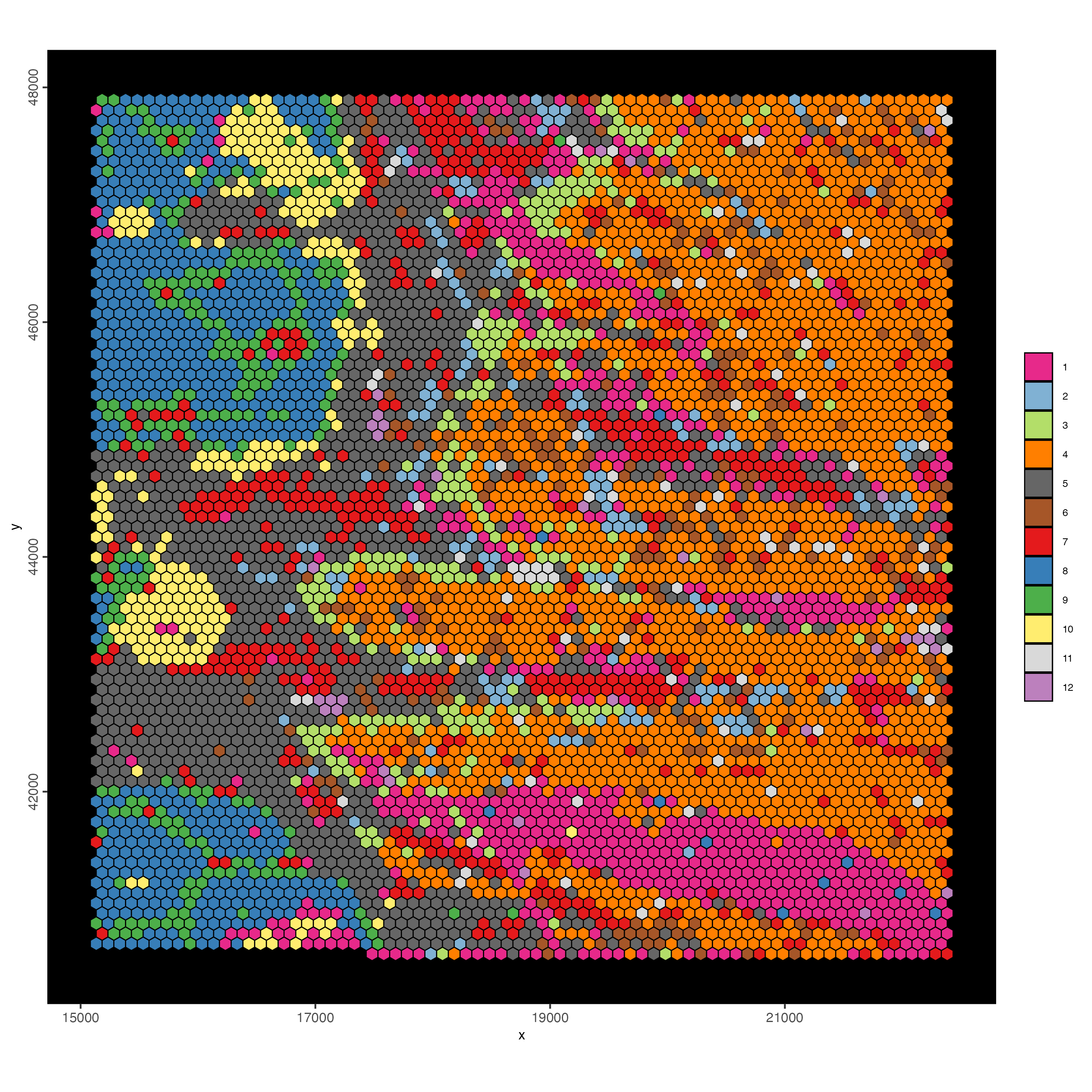
spatInSituPlotPoints(visiumHD,
    show_image = FALSE,
    feats = NULL,
    show_legend = FALSE,
    spat_unit = "hex100",
    point_size = 0.5,
    show_polygon = TRUE,
    use_overlap = FALSE,
    polygon_feat_type = "hex100",
    polygon_fill_as_factor = TRUE,
    polygon_fill = "leiden_clus",
    polygon_color = "black",
    polygon_line_size = 0.3
)
6.2 Spatial expression patterns
6.2.1 Identify single genes
Here we will use binSpect as a quick method to rank genes with high potential for spatial coherent expression patterns.
featData <- fDataDT(visiumHD,
spat_unit = "hex100"
)
hvf_genes <- featData[hvf == "yes"]$feat_ID
visiumHD <- createSpatialNetwork(visiumHD,
name = "kNN_network",
spat_unit = "hex100",
method = "kNN",
k = 8
)
ranktest <- binSpect(visiumHD,
spat_unit = "hex100",
subset_feats = hvf_genes,
bin_method = "rank",
calc_hub = FALSE,
do_fisher_test = TRUE,
spatial_network_name = "kNN_network"
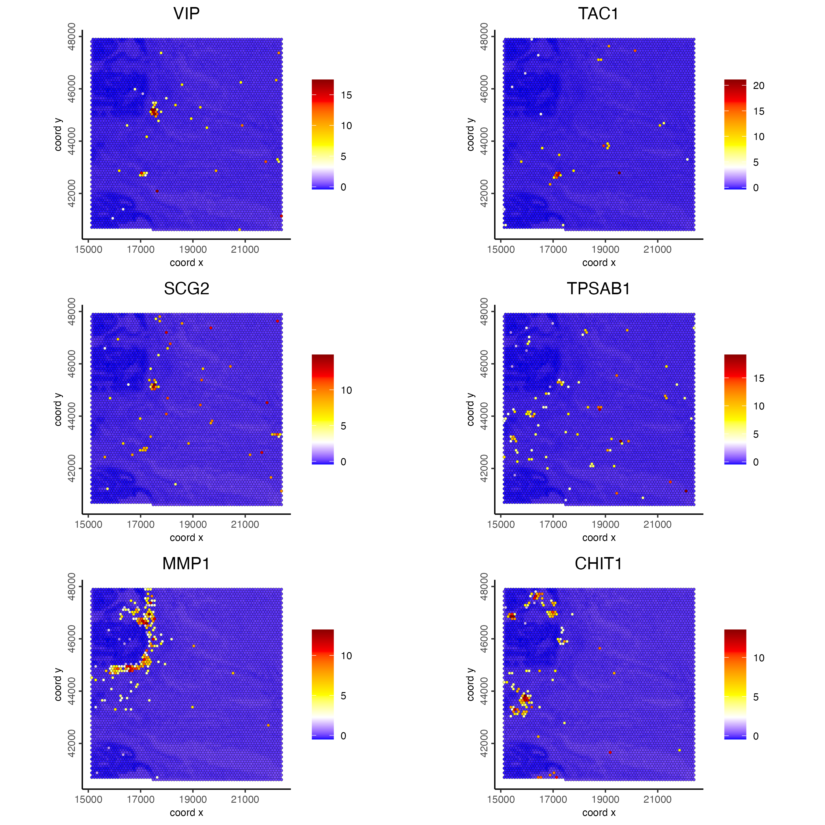
)Visualize top 2 ranked spatial genes per expression bin:
set0 <- ranktest[high_expr < 50][1:2]$feats
set1 <- ranktest[high_expr > 50 & high_expr < 100][1:2]$feats
set2 <- ranktest[high_expr > 100 & high_expr < 200][1:2]$feats
set3 <- ranktest[high_expr > 200 & high_expr < 400][1:2]$feats
set4 <- ranktest[high_expr > 400 & high_expr < 1000][1:2]$feats
set5 <- ranktest[high_expr > 1000][1:2]$feats

spatFeatPlot2D(visiumHD,
    spat_unit = "hex100",
    expression_values = "scaled",
    feats = c(set0, set1, set2),
    gradient_style = "sequential",
    cell_color_gradient = c("blue", "white", "yellow", "orange", "red", "darkred"),
    cow_n_col = 2, point_size = 1
)
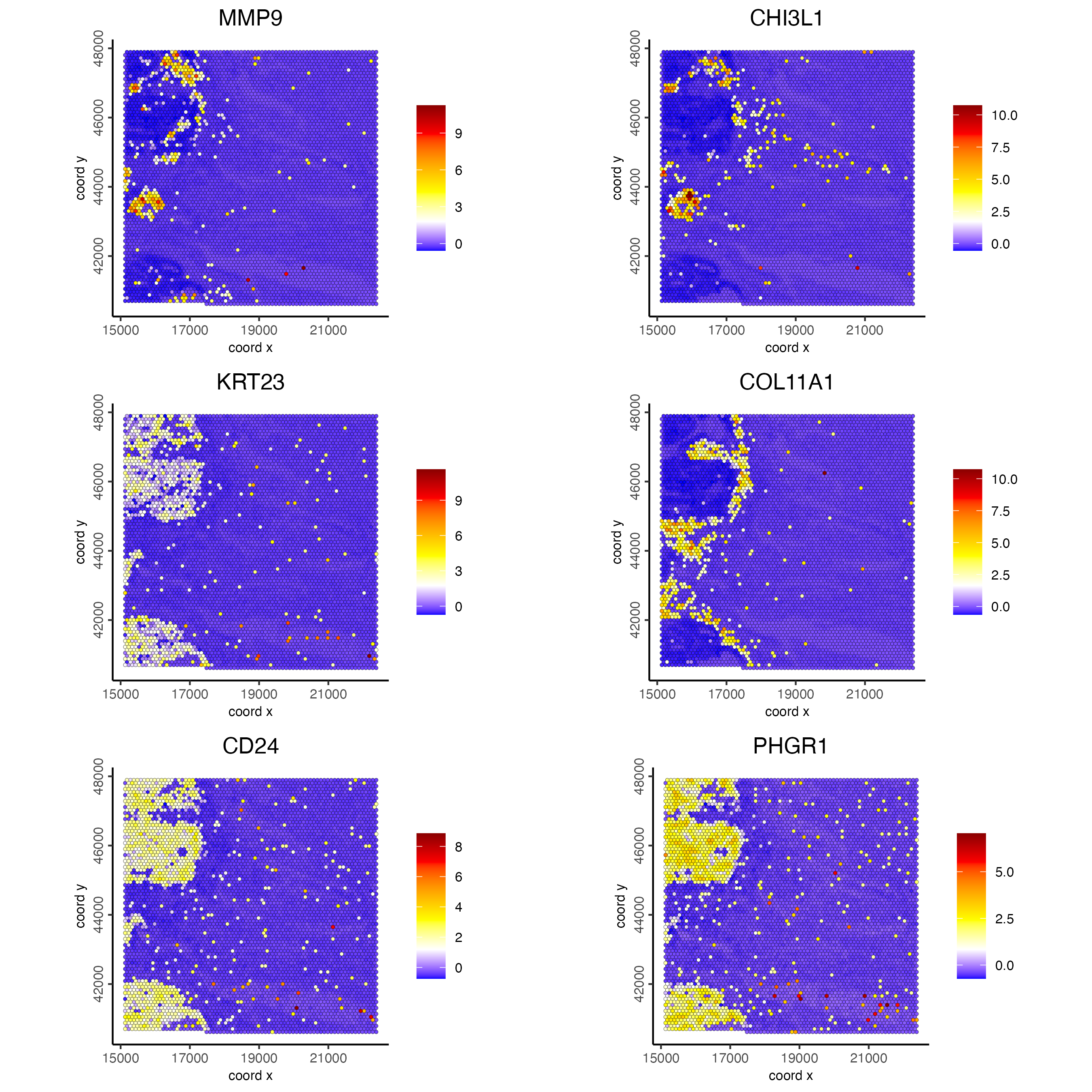
spatFeatPlot2D(visiumHD,
    spat_unit = "hex100",
    expression_values = "scaled",
    feats = c(set3, set4, set5),
    gradient_style = "sequential",
    cell_color_gradient = c("blue", "white", "yellow", "orange", "red", "darkred"),
    cow_n_col = 2, point_size = 1
)
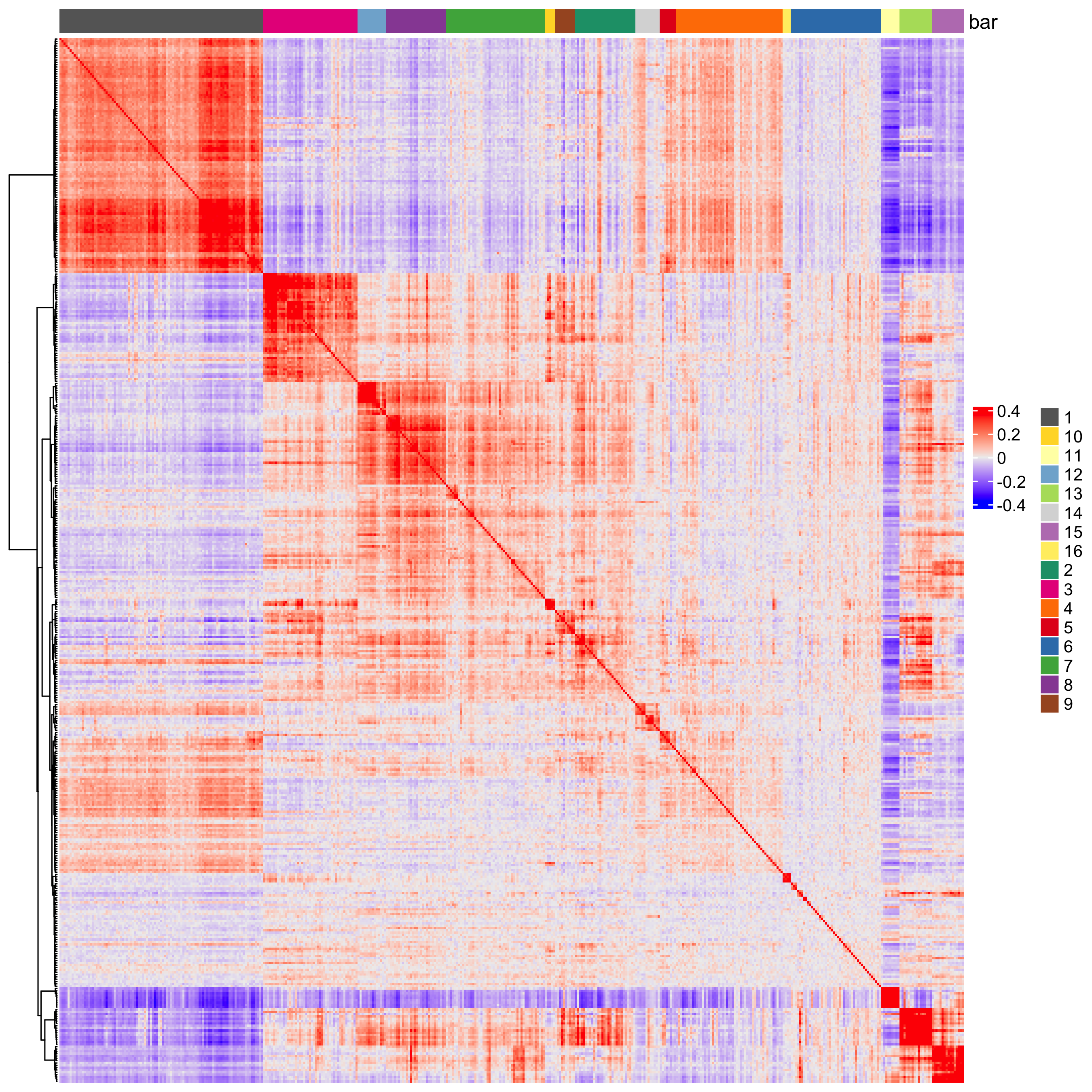
6.2.2 Spatial co-expression modules
Investigating individual genes is a good start, but here we would like to identify recurrent spatial expression patterns that are shared by spatial co-expression modules that might represent spatially organized biological processes.
ext_spatial_genes <- ranktest[adj.p.value < 0.001]$feats

spat_cor_netw_DT <- detectSpatialCorFeats(visiumHD,
    spat_unit = "hex100",
    method = "network",
    spatial_network_name = "kNN_network",
    subset_feats = ext_spatial_genes
)

# cluster spatial genes
spat_cor_netw_DT <- clusterSpatialCorFeats(spat_cor_netw_DT,
    name = "spat_netw_clus",
    k = 16
)

# visualize clusters
heatmSpatialCorFeats(visiumHD,
    spatCorObject = spat_cor_netw_DT,
    use_clus_name = "spat_netw_clus",
    heatmap_legend_param = list(title = NULL)
)
# create metagene enrichment score for clusters
cluster_genes_DT <- showSpatialCorFeats(spat_cor_netw_DT,
    use_clus_name = "spat_netw_clus",
    show_top_feats = 1
)

cluster_genes <- cluster_genes_DT$clus
names(cluster_genes) <- cluster_genes_DT$feat_ID

visiumHD <- createMetafeats(visiumHD,
    spat_unit = "hex100",
    expression_values = "normalized",
    feat_clusters = cluster_genes,
    name = "cluster_metagene"
)

showGiottoSpatEnrichments(visiumHD)
spatCellPlot(visiumHD,
    spat_unit = "hex100",
    spat_enr_names = "cluster_metagene",
    gradient_style = "sequential",
    cell_color_gradient = c("blue", "white", "yellow", "orange", "red", "darkred"),
    cell_annotation_values = as.character(c(1:4)),
    point_size = 1, cow_n_col = 2
)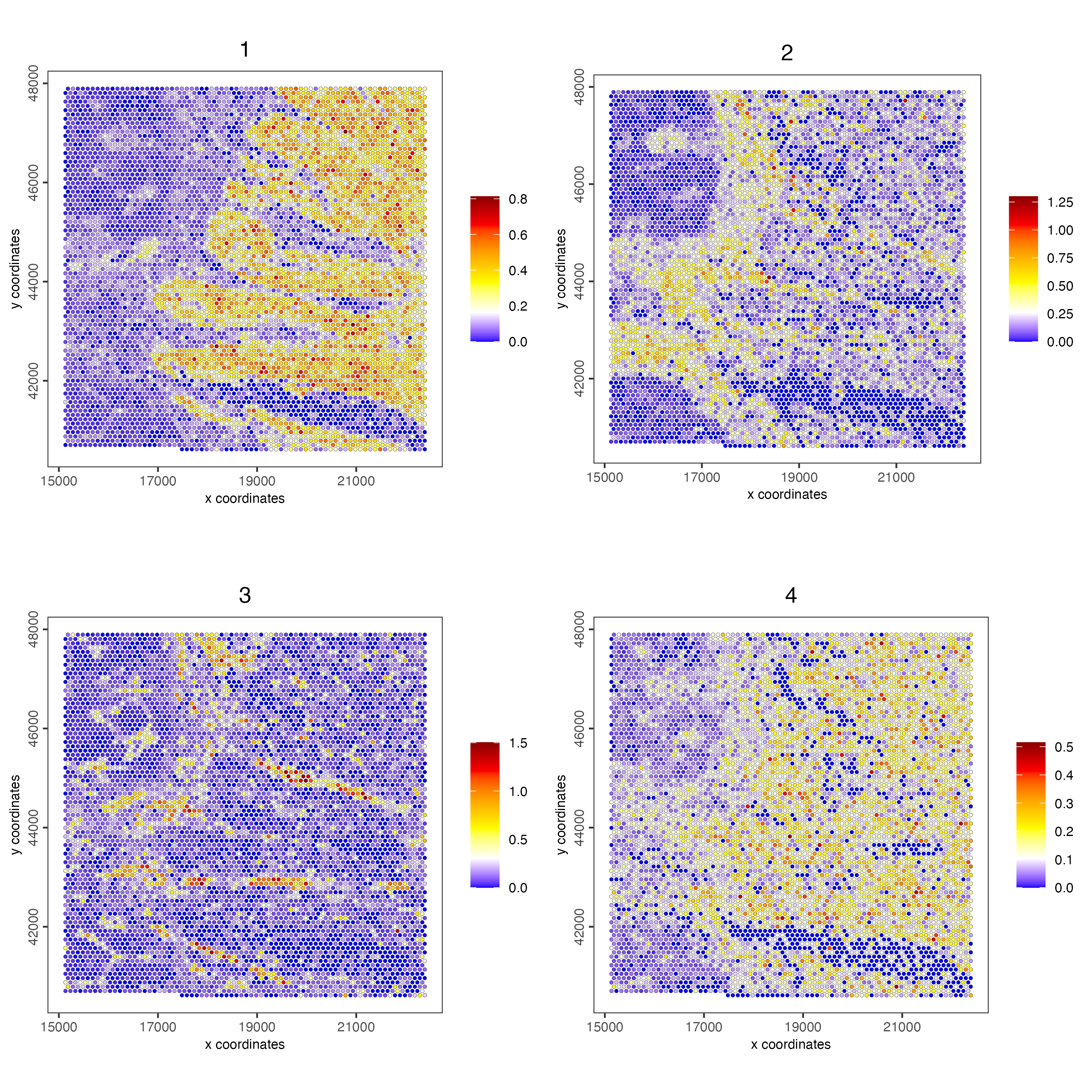
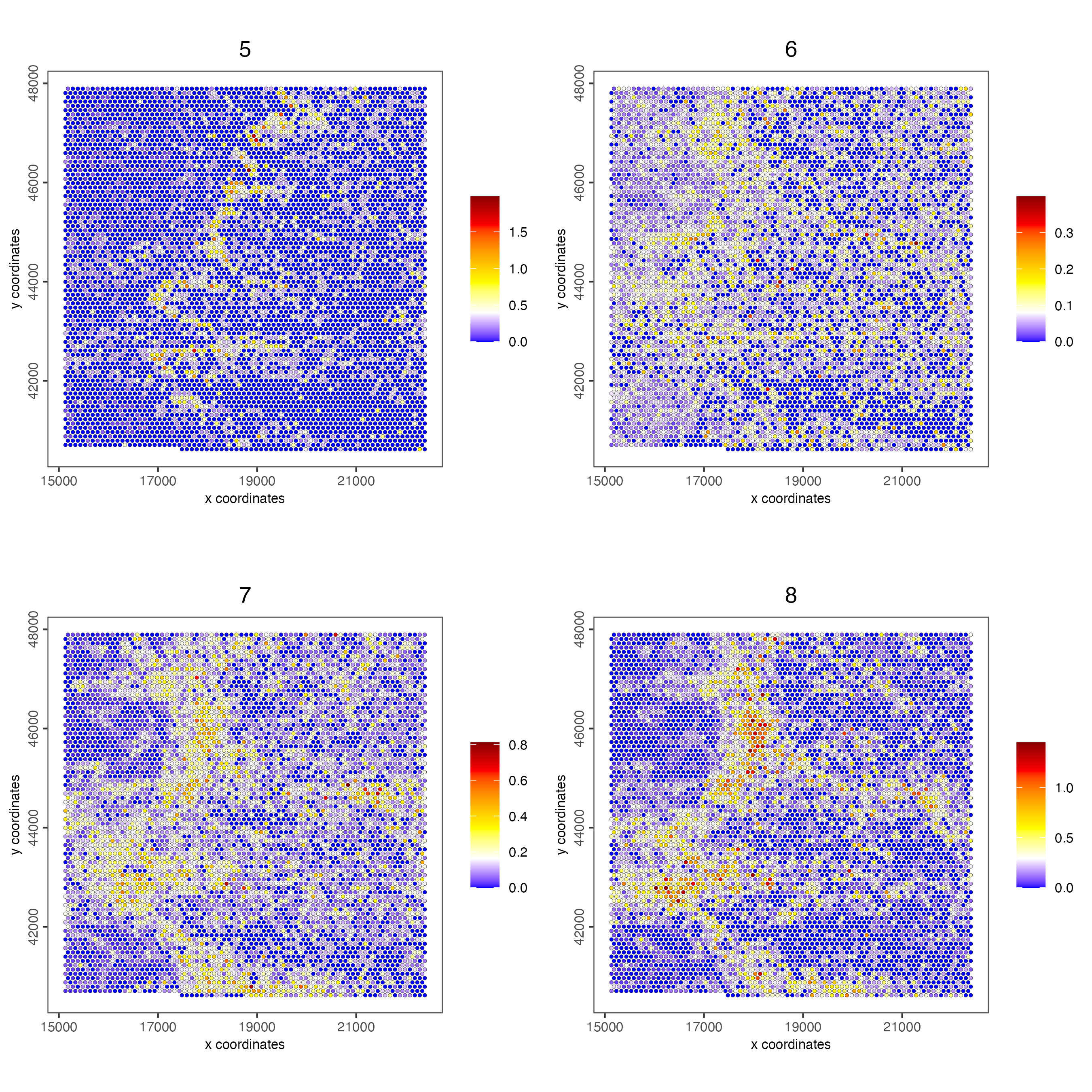
spatCellPlot(visiumHD,
    spat_unit = "hex100",
    spat_enr_names = "cluster_metagene",
    gradient_style = "sequential",
    cell_color_gradient = c("blue", "white", "yellow", "orange", "red", "darkred"),
    cell_annotation_values = as.character(c(5:8)),
    point_size = 1, cow_n_col = 2
)
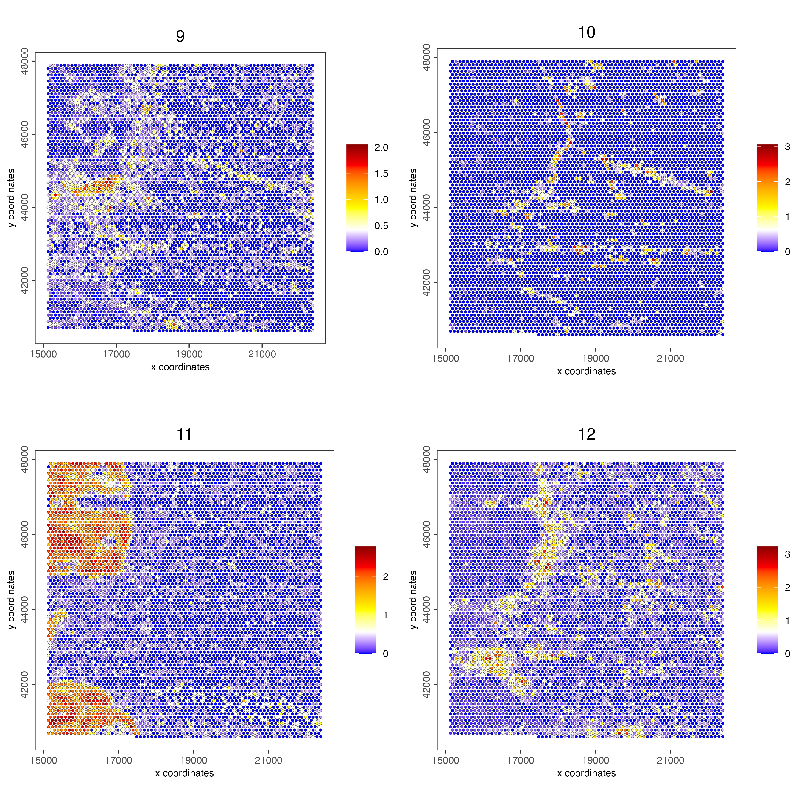
spatCellPlot(visiumHD,
    spat_unit = "hex100",
    spat_enr_names = "cluster_metagene",
    gradient_style = "sequential",
    cell_color_gradient = c("blue", "white", "yellow", "orange", "red", "darkred"),
    cell_annotation_values = as.character(c(9:12)),
    point_size = 1, cow_n_col = 2
)
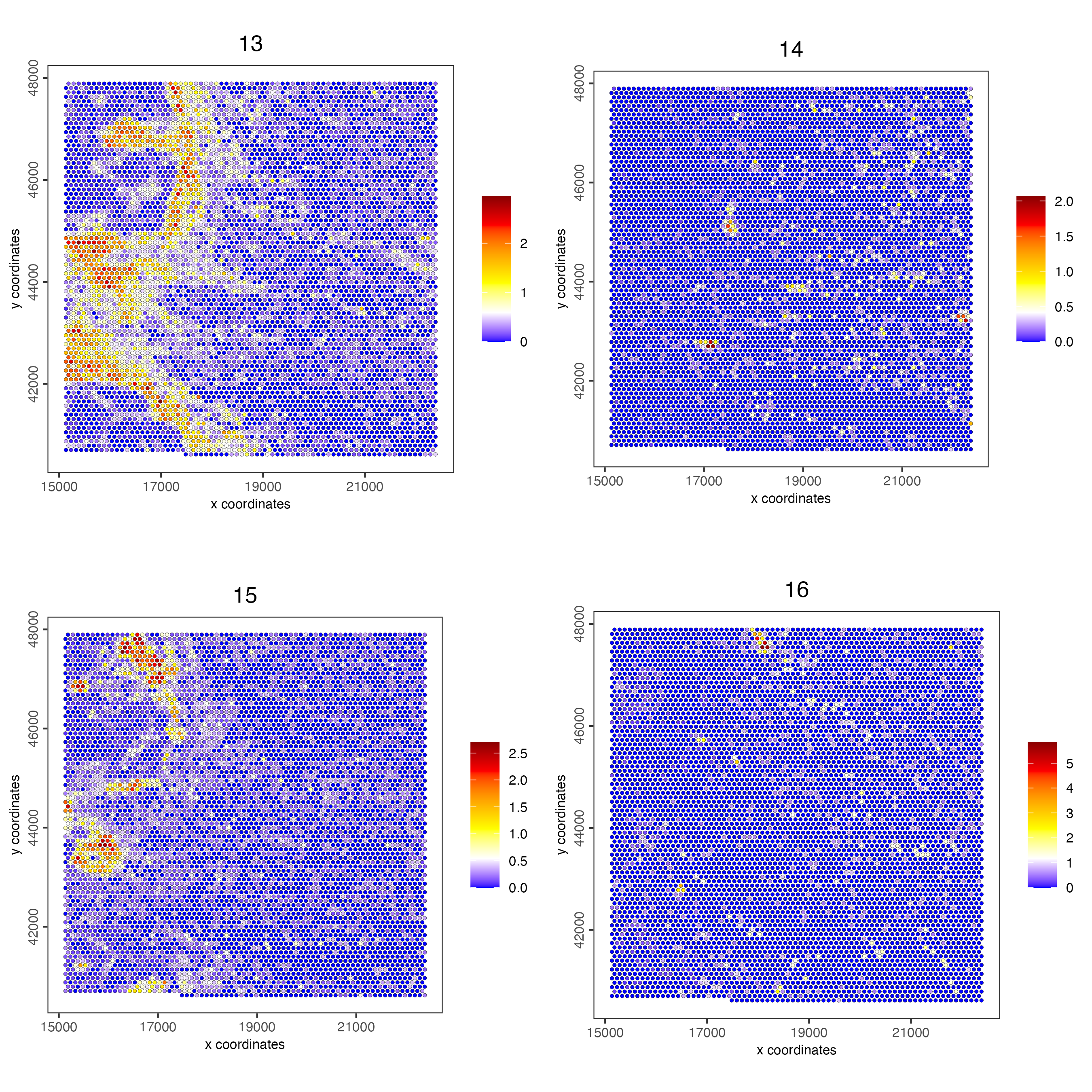
spatCellPlot(visiumHD,
    spat_unit = "hex100",
    spat_enr_names = "cluster_metagene",
    gradient_style = "sequential",
    cell_color_gradient = c("blue", "white", "yellow", "orange", "red", "darkred"),
    cell_annotation_values = as.character(c(13:16)),
    point_size = 1, cow_n_col = 2
)
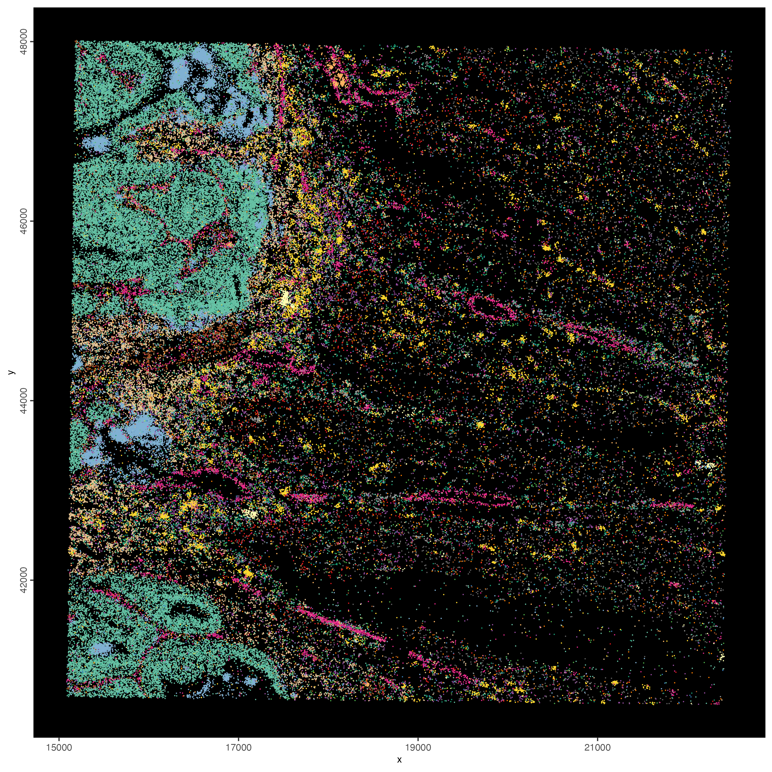
6.2.3 Plot spatial gene groups
Hack! Vendors of spatial technologies typically like to show very interesting spatial gene expression patterns. Here we will follow a similar strategy by selecting a balanced set of genes for each spatial co-expression module and then to simply give them the same color in the spatInSituPlotPoints function.
balanced_genes <- getBalancedSpatCoexpressionFeats(
    spatCorObject = spat_cor_netw_DT,
    maximum = 5
)
selected_feats <- names(balanced_genes)

# give genes from same cluster same color
distinct_colors <- getDistinctColors(n = 20)
names(distinct_colors) <- 1:20

my_colors <- distinct_colors[balanced_genes]
names(my_colors) <- names(balanced_genes)

spatInSituPlotPoints(visiumHD,
    spat_unit = "hex100",
    show_image = FALSE,
    feats = list("rna" = selected_feats),
    feats_color_code = my_colors,
    show_legend = FALSE,
    point_size = 0.20,
    show_polygon = FALSE,
    use_overlap = FALSE,
    polygon_feat_type = "hex100",
    polygon_bg_color = NA,
    polygon_color = "white",
    polygon_line_size = 0.01,
    expand_counts = TRUE,
    count_info_column = "count",
    jitter = c(25, 25)
)
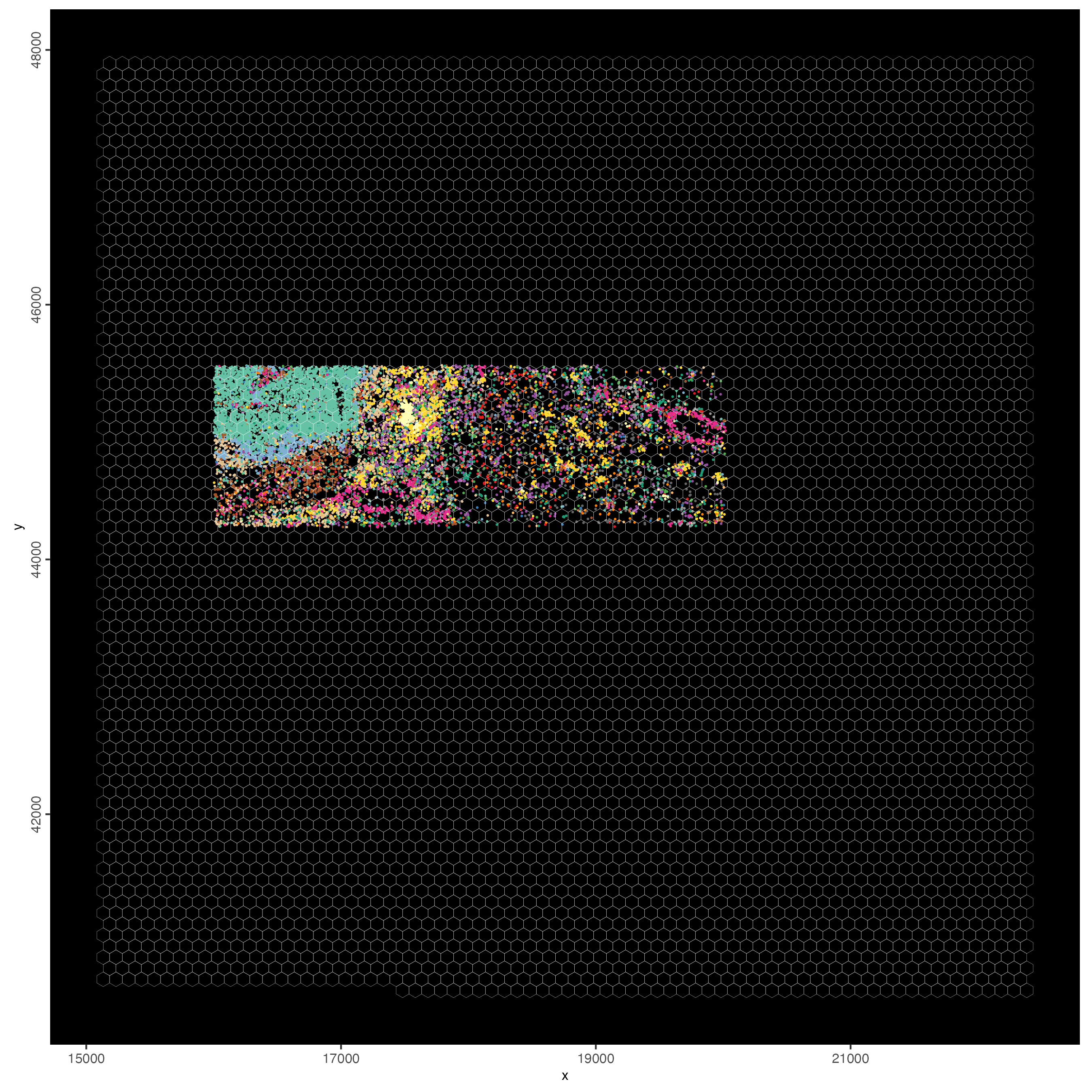
7 Hexbin 25
The goal is to create a higher resolution bin (hex25) and add to the Giotto object. We will aim to identify individual cell types and local neighborhood niches.
7.1 Subcellular workflow
visiumHD_subset <- subsetGiottoLocs(
    gobject = visiumHD,
    x_min = 16000,
    x_max = 20000,
    y_min = 44250,
    y_max = 45500
)
Plot visiumHD subset with hexbin100 polygons:
spatInSituPlotPoints(visiumHD_subset,
    spat_unit = "hex100",
    show_image = FALSE,
    feats = NULL,
    show_legend = FALSE,
    point_size = 0.5,
    show_polygon = TRUE,
    use_overlap = FALSE,
    polygon_feat_type = "hex100",
    polygon_fill_as_factor = TRUE,
    polygon_fill = "leiden_clus",
    polygon_color = "black",
    polygon_line_size = 0.3
)
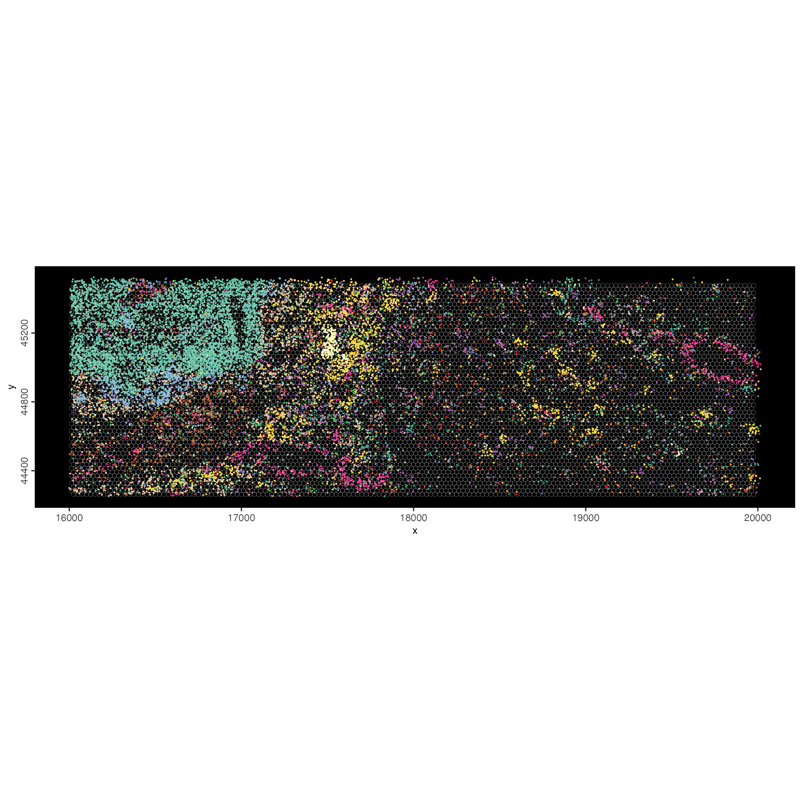
Plot visiumHD subset with selected gene features:
spatInSituPlotPoints(visiumHD_subset,
    spat_unit = "hex100",
    show_image = FALSE,
    feats = list("rna" = selected_feats),
    feats_color_code = my_colors,
    show_legend = FALSE,
    point_size = 0.40,
    show_polygon = TRUE,
    use_overlap = FALSE,
    polygon_feat_type = "hex100",
    polygon_bg_color = NA,
    polygon_color = "white",
    polygon_line_size = 0.05,
    jitter = c(25, 25)
)
Create smaller hexbin25 tessellations:
hexbin25 <- tessellate(
    extent = ext(visiumHD_subset@feat_info$rna),
    shape = "hexagon",
    shape_size = 25,
    name = "hex25"
)

visiumHD_subset <- setPolygonInfo(
    gobject = visiumHD_subset,
    x = hexbin25,
    name = "hex25",
    initialize = TRUE
)

showGiottoSpatialInfo(visiumHD_subset)

visiumHD_subset <- addSpatialCentroidLocations(
    gobject = visiumHD_subset,
    poly_info = "hex25"
)

activeSpatUnit(visiumHD_subset) <- "hex25"

spatInSituPlotPoints(visiumHD_subset,
    spat_unit = "hex25",
    show_image = FALSE,
    feats = list("rna" = selected_feats),
    feats_color_code = my_colors,
    show_legend = FALSE,
    point_size = 0.40,
    show_polygon = TRUE,
    use_overlap = FALSE,
    polygon_feat_type = "hex25",
    polygon_bg_color = NA,
    polygon_color = "white",
    polygon_line_size = 0.05,
    jitter = c(25, 25)
)
visiumHD_subset <- calculateOverlap(visiumHD_subset,
    spatial_info = "hex25",
    feat_info = "rna"
)

showGiottoSpatialInfo(visiumHD_subset)

# convert overlap results to bin by gene matrix
visiumHD_subset <- overlapToMatrix(visiumHD_subset,
    poly_info = "hex25",
    feat_info = "rna",
    name = "raw"
)

visiumHD_subset <- filterGiotto(visiumHD_subset,
    expression_threshold = 1,
    feat_det_in_min_cells = 3,
    min_det_feats_per_cell = 5
)

activeSpatUnit(visiumHD_subset)


# normalize
visiumHD_subset <- normalizeGiotto(visiumHD_subset,
    scalefactor = 1000,
    verbose = TRUE
)

# add statistics
visiumHD_subset <- addStatistics(visiumHD_subset)

feature_data <- fDataDT(visiumHD_subset)

visiumHD_subset <- calculateHVF(visiumHD_subset,
    zscore_threshold = 1
)
n_25_percent <- round(length(spatIDs(visiumHD_subset, "hex25")) * 0.25)
# pca projection on subset
visiumHD_subset <- runPCAprojection(
gobject = visiumHD_subset,
spat_unit = "hex25",
feats_to_use = "hvf",
name = "pca.projection",
set_seed = TRUE,
seed_number = 12345,
random_subset = n_25_percent
)
showGiottoDimRed(visiumHD_subset)
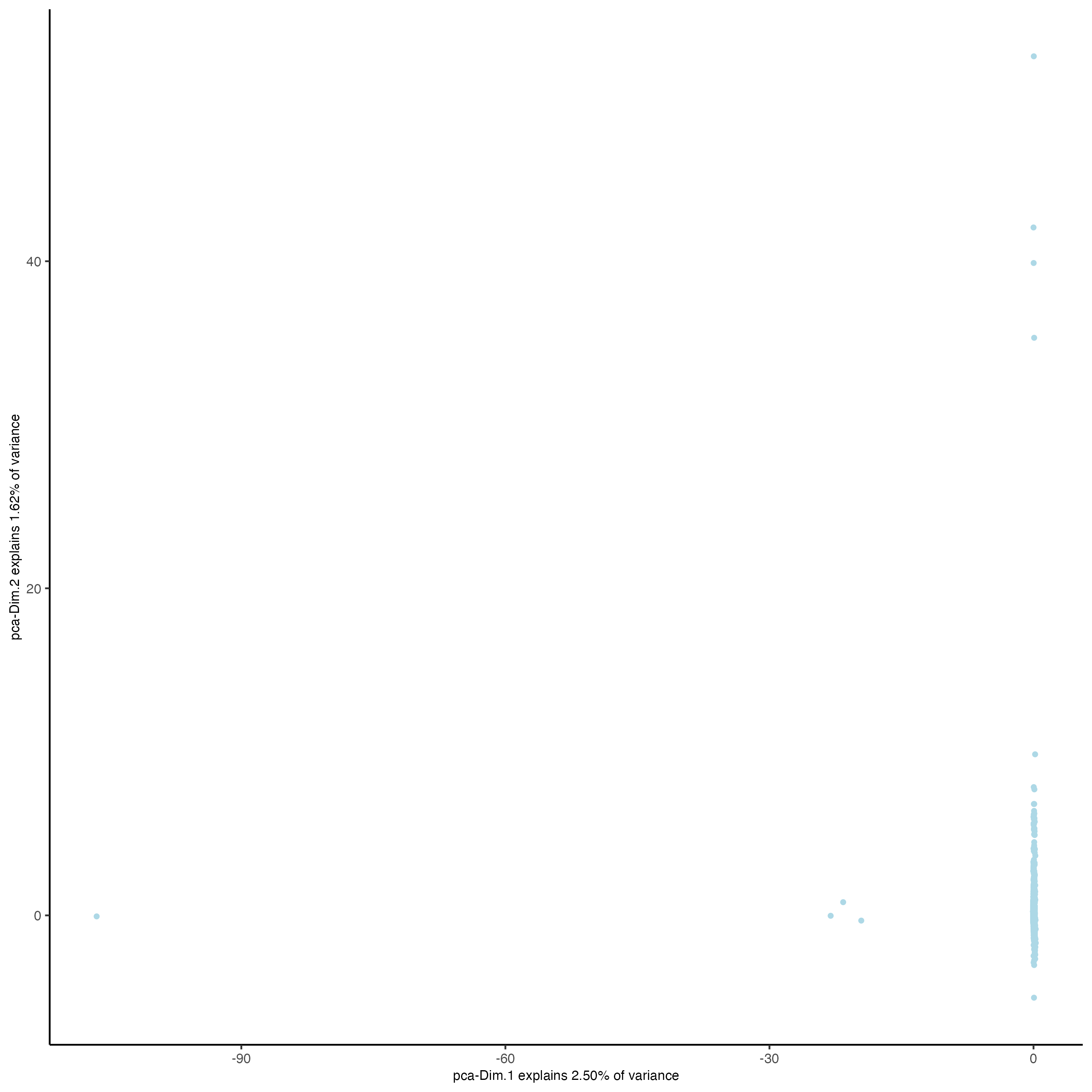
plotPCA(visiumHD_subset,
spat_unit = "hex25",
dim_reduction_name = "pca.projection"
)
# umap projection on subset
visiumHD_subset <- runUMAPprojection(
gobject = visiumHD_subset,
spat_unit = "hex25",
dim_reduction_to_use = "pca",
dim_reduction_name = "pca.projection",
dimensions_to_use = 1:10,
name = "umap.projection",
random_subset = n_25_percent,
n_neighbors = 10,
min_dist = 0.005,
n_threads = 4
)
showGiottoDimRed(visiumHD_subset)
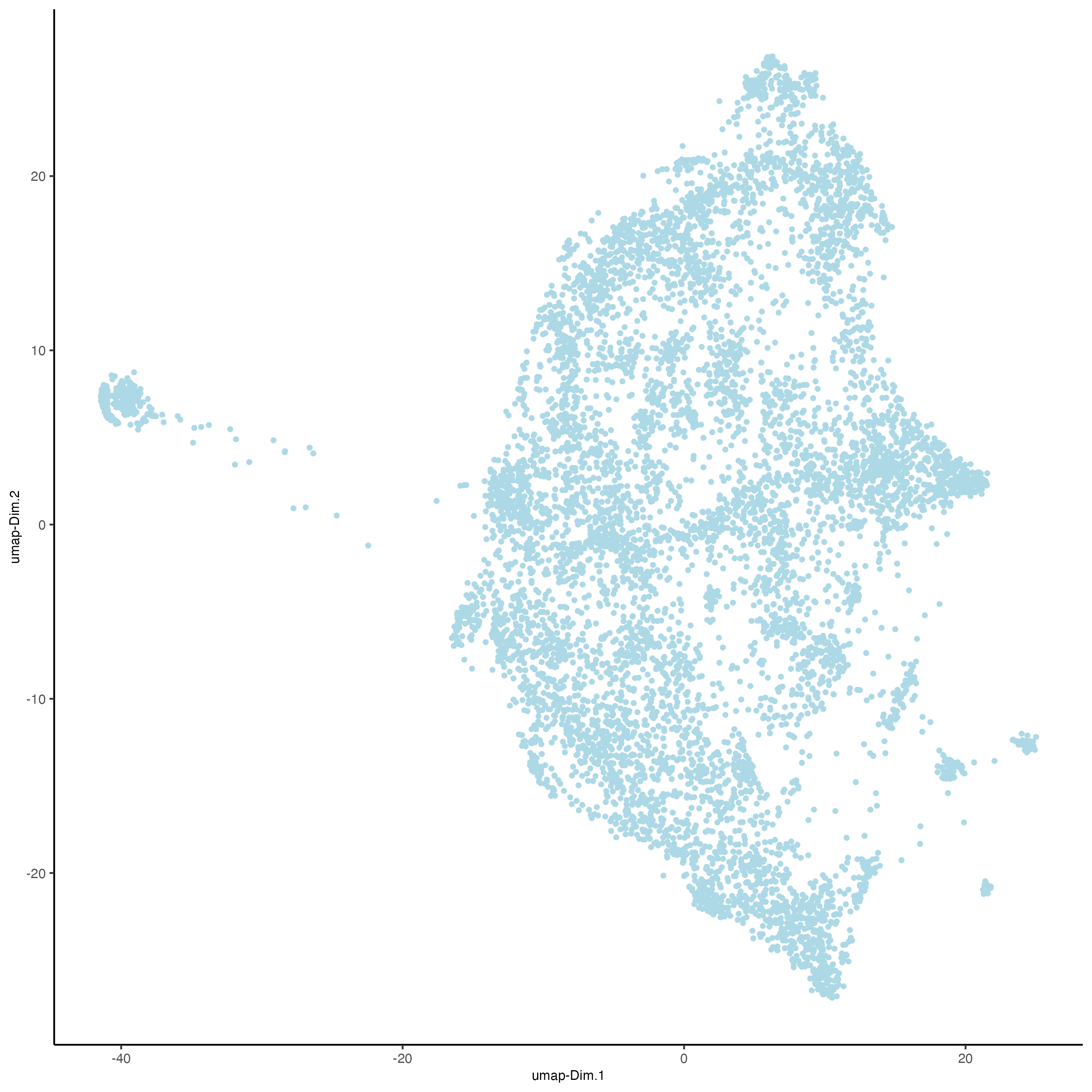
# plot UMAP, coloring cells/points based on nr_feats
plotUMAP(
gobject = visiumHD_subset,
point_size = 1,
dim_reduction_name = "umap.projection"
)
7.2 Clustering with projection
- subsample Giotto object
- perform clustering (e.g. hierarchical clustering)
- project cluster results to full Giotto object using a kNN voting approach and a shared dimension reduction space (e.g. PCA)
# subset to smaller giotto object
set.seed(1234)
subset_IDs <- sample(x = spatIDs(visiumHD_subset, "hex25"), size = n_25_percent)
temp_gobject <- subsetGiotto(
gobject = visiumHD_subset,
spat_unit = "hex25",
cell_ids = subset_IDs
)
# hierarchical clustering
temp_gobject <- doHclust(
gobject = temp_gobject,
spat_unit = "hex25",
k = 8, name = "sub_hclust",
dim_reduction_to_use = "pca",
dim_reduction_name = "pca.projection",
dimensions_to_use = 1:10
)
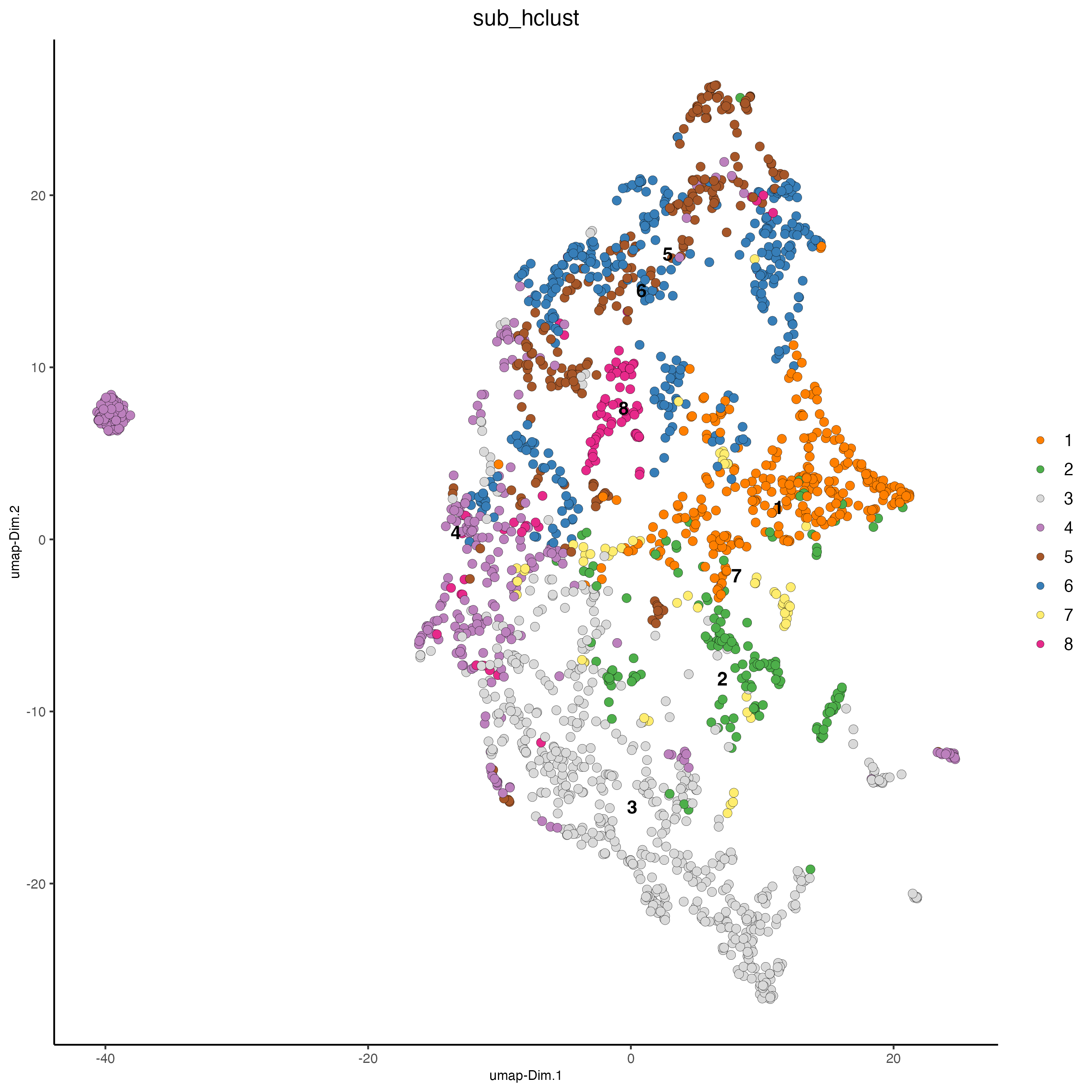
# show umap
dimPlot2D(
gobject = temp_gobject,
point_size = 2.5,
spat_unit = "hex25",
dim_reduction_to_use = "umap",
dim_reduction_name = "umap.projection",
cell_color = "sub_hclust"
)
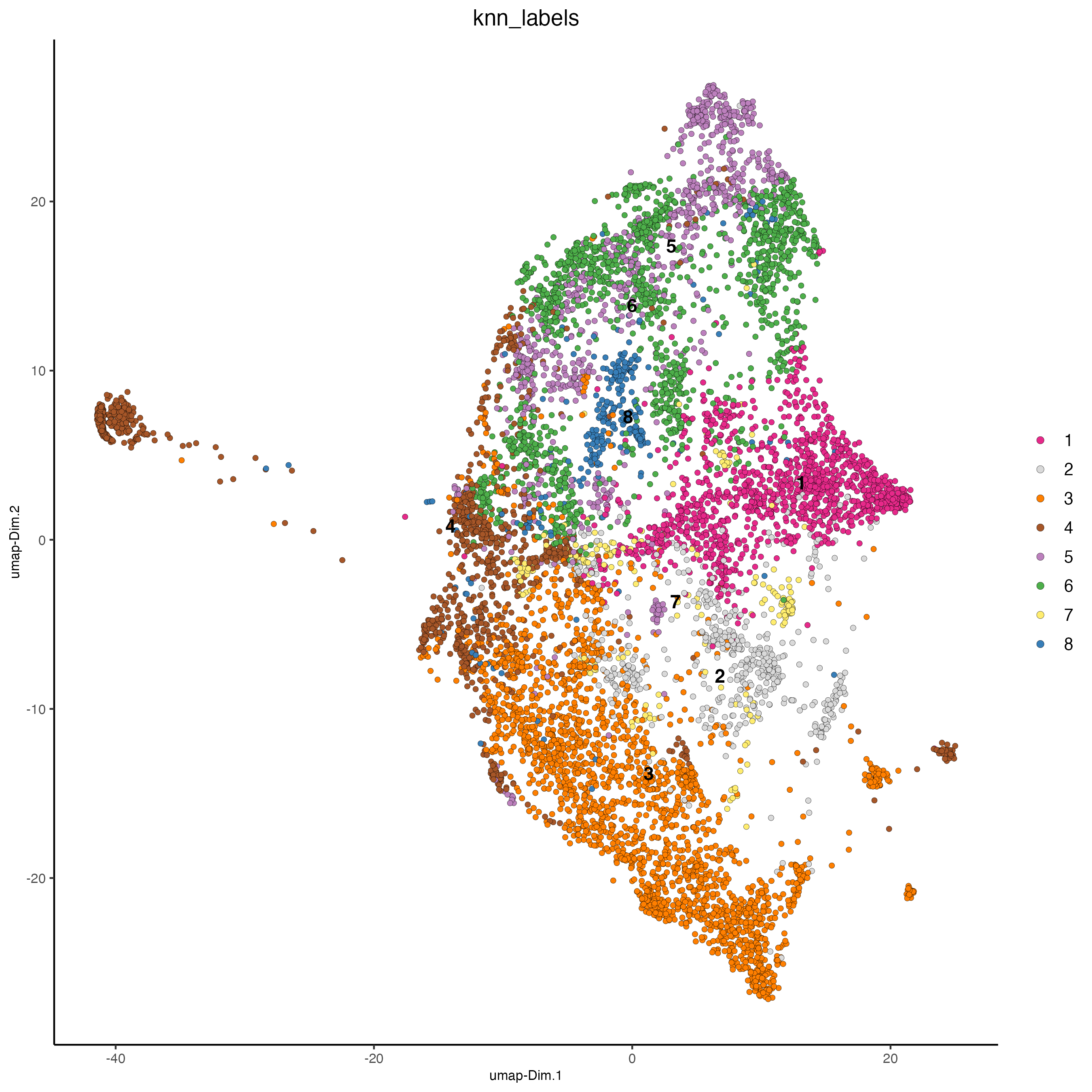
# project clusterings back to full dataset
visiumHD_subset <- labelTransfer(
    x = visiumHD_subset,
    y = temp_gobject,
    spat_unit = "hex25",
    labels = "sub_hclust",
    reduction_method = "pca",
    reduction_name = "pca.projection",
    prob = FALSE,
    k = 5,
    dimensions_to_use = 1:10
)

pDataDT(visiumHD_subset)

dimPlot2D(
    gobject = visiumHD_subset,
    point_size = 1.5,
    spat_unit = "hex25",
    dim_reduction_to_use = "umap",
    dim_reduction_name = "umap.projection",
    cell_color = "knn_labels"
)
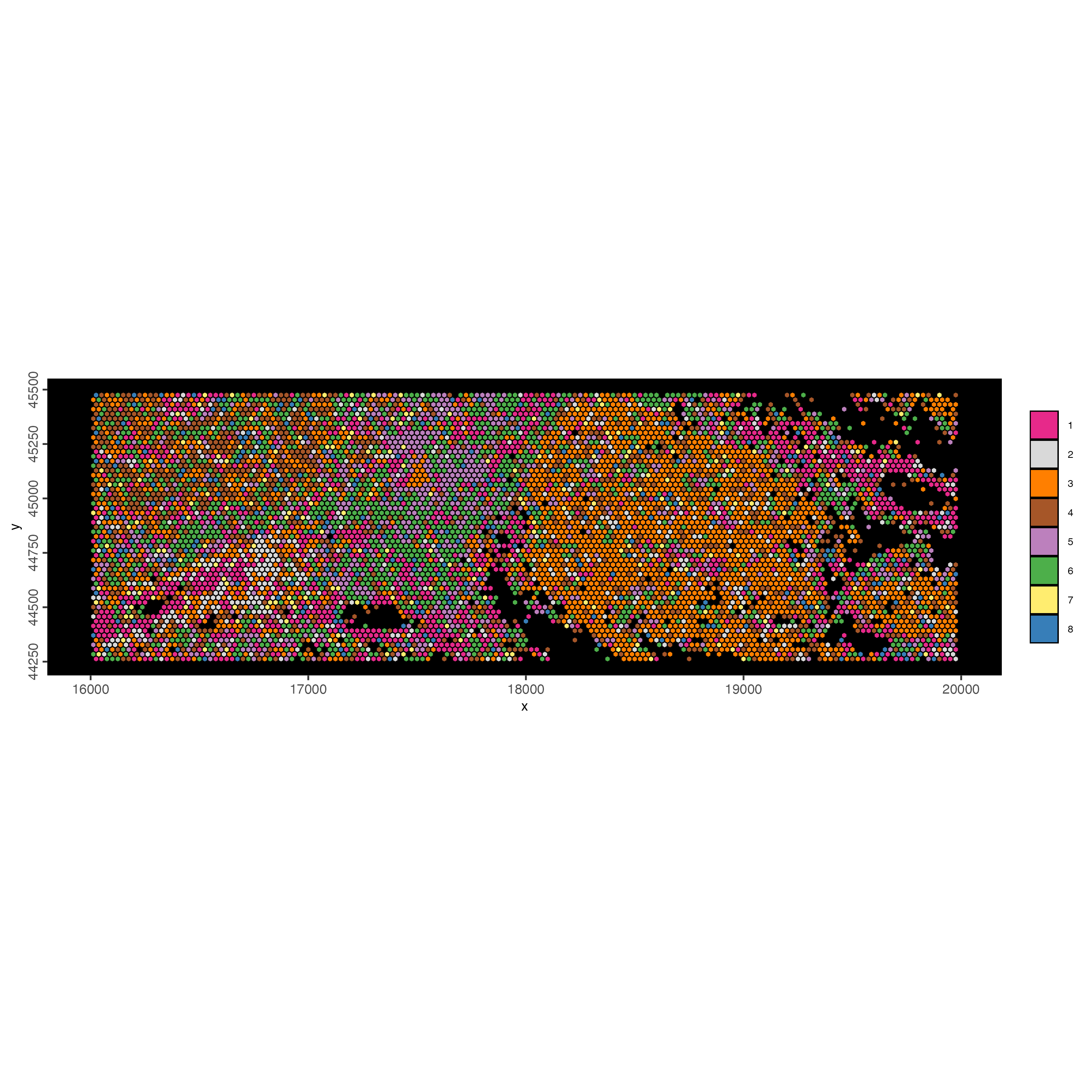
spatInSituPlotPoints(visiumHD_subset,
    show_image = FALSE,
    feats = NULL,
    show_legend = FALSE,
    spat_unit = "hex25",
    point_size = 0.5,
    show_polygon = TRUE,
    use_overlap = FALSE,
    polygon_feat_type = "hex25",
    polygon_fill_as_factor = TRUE,
    polygon_fill = "knn_labels",
    polygon_color = "black",
    polygon_line_size = 0.3
)
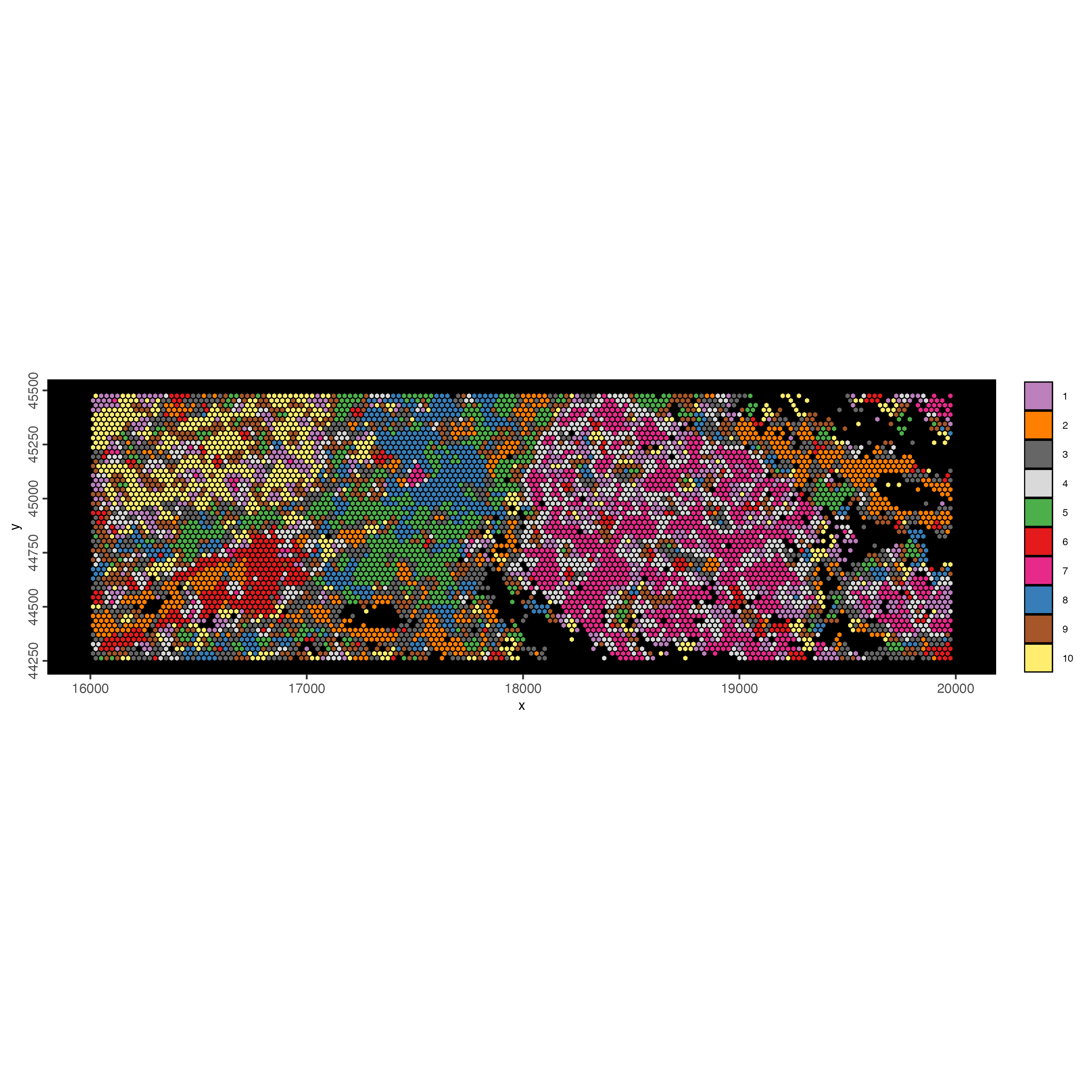
7.3 Niche clustering
Each cell will be clustered based on its neighboring cell type composition. Size of cellular niche is important and defines the tissue organization resolution.
visiumHD_subset <- createSpatialNetwork(visiumHD_subset,
    name = "kNN_network",
    spat_unit = "hex25",
    method = "kNN",
    k = 6
)

pDataDT(visiumHD_subset)

visiumHD_subset <- calculateSpatCellMetadataProportions(
    gobject = visiumHD_subset,
    spat_unit = "hex25",
    feat_type = "rna",
    metadata_column = "knn_labels",
    spat_network = "kNN_network"
)

prop_table <- getSpatialEnrichment(visiumHD_subset,
                                   name = "proportion",
                                   output = "data.table")

prop_matrix <- GiottoUtils:::dt_to_matrix(prop_table)

set.seed(1234)
prop_kmeans <- kmeans(x = prop_matrix,
                      centers = 10,
                      iter.max = 1000,
                      nstart = 100)

prop_kmeansDT <- data.table::data.table(cell_ID = names(prop_kmeans$cluster),
                                        niche = prop_kmeans$cluster)

visiumHD_subset <- addCellMetadata(visiumHD_subset,
    new_metadata = prop_kmeansDT,
    by_column = TRUE,
    column_cell_ID = "cell_ID"
)

pDataDT(visiumHD_subset)

spatInSituPlotPoints(visiumHD_subset,
    show_image = FALSE,
    feats = NULL,
    show_legend = FALSE,
    spat_unit = "hex25",
    point_size = 0.5,
    show_polygon = TRUE,
    use_overlap = FALSE,
    polygon_feat_type = "hex25",
    polygon_fill_as_factor = TRUE,
    polygon_fill = "niche",
    polygon_color = "black",
    polygon_line_size = 0.3
)
8 Session info
R version 4.4.2 (2024-10-31)
Platform: x86_64-apple-darwin20
Running under: macOS Sequoia 15.3

Matrix products: default
BLAS:   /System/Library/Frameworks/Accelerate.framework/Versions/A/Frameworks/vecLib.framework/Versions/A/libBLAS.dylib
LAPACK: /Library/Frameworks/R.framework/Versions/4.4-x86_64/Resources/lib/libRlapack.dylib;  LAPACK version 3.12.0

locale:
[1] en_US.UTF-8/en_US.UTF-8/en_US.UTF-8/C/en_US.UTF-8/en_US.UTF-8

time zone: America/New_York
tzcode source: internal

attached base packages:
[1] stats     graphics  grDevices utils     datasets  methods   base

other attached packages:
[1] Giotto_4.2.1      GiottoClass_0.4.7

loaded via a namespace (and not attached):
  [1] RColorBrewer_1.1-3          shape_1.4.6.1               rstudioapi_0.17.1
  [4] jsonlite_1.8.9              magrittr_2.0.3              magick_2.8.5
  [7] farver_2.1.2                rmarkdown_2.29              GlobalOptions_0.1.2
 [10] fs_1.6.5                    zlibbioc_1.52.0             ragg_1.3.3
 [13] vctrs_0.6.5                 Cairo_1.6-2                 GiottoUtils_0.2.4
 [16] terra_1.8-15                htmltools_0.5.8.1           S4Arrays_1.6.0
 [19] usethis_3.1.0               curl_6.2.0                  SparseArray_1.6.0
 [22] parallelly_1.41.0           htmlwidgets_1.6.4           desc_1.4.3
 [25] plotly_4.10.4               igraph_2.1.4                lifecycle_1.0.4
 [28] iterators_1.0.14            pkgconfig_2.0.3             rsvd_1.0.5
 [31] Matrix_1.7-2                R6_2.5.1                    fastmap_1.2.0
 [34] clue_0.3-66                 GenomeInfoDbData_1.2.13     MatrixGenerics_1.18.0
 [37] future_1.34.0               digest_0.6.37               colorspace_2.1-1
 [40] S4Vectors_0.44.0            ps_1.8.1                    irlba_2.3.5.1
 [43] textshaping_1.0.0           GenomicRanges_1.58.0        beachmat_2.22.0
 [46] labeling_0.4.3              httr_1.4.7                  abind_1.4-8
 [49] compiler_4.4.2              remotes_2.5.0               bit64_4.6.0-1
 [52] withr_3.0.2                 doParallel_1.0.17           backports_1.5.0
 [55] BiocParallel_1.40.0         pkgbuild_1.4.6              R.utils_2.12.3
 [58] DelayedArray_0.32.0         rjson_0.2.23                gtools_3.9.5
 [61] GiottoVisuals_0.2.12        tools_4.4.2                 future.apply_1.11.3
 [64] R.oo_1.27.0                 glue_1.8.0                  dbscan_1.2-0
 [67] callr_3.7.6                 R.cache_0.16.0              grid_4.4.2
 [70] checkmate_2.3.2             cluster_2.1.8               generics_0.1.3
 [73] gtable_0.3.6                R.methodsS3_1.8.2           tidyr_1.3.1
 [76] data.table_1.16.4           BiocSingular_1.22.0         ScaledMatrix_1.14.0
 [79] XVector_0.46.0              BiocGenerics_0.52.0         RcppAnnoy_0.0.22
 [82] ggrepel_0.9.6               foreach_1.5.2               pillar_1.10.1
 [85] circlize_0.4.16             dplyr_1.1.4                 lattice_0.22-6
 [88] FNN_1.1.4.1                 bit_4.5.0.1                 tidyselect_1.2.1
 [91] ComplexHeatmap_2.22.0       SingleCellExperiment_1.28.1 knitr_1.49
 [94] biocthis_1.16.0             IRanges_2.40.1              SummarizedExperiment_1.36.0
 [97] scattermore_1.2             stats4_4.4.2                xfun_0.50
[100] Biobase_2.66.0              matrixStats_1.5.0           UCSC.utils_1.2.0
[103] lazyeval_0.2.2              yaml_2.3.10                 evaluate_1.0.3
[106] codetools_0.2-20            tibble_3.2.1                colorRamp2_0.1.0
[109] cli_3.6.3                   uwot_0.2.2                  arrow_18.1.0.1
[112] reticulate_1.40.0           systemfonts_1.2.1           munsell_0.5.1
[115] processx_3.8.5              styler_1.10.3               Rcpp_1.0.14
[118] GenomeInfoDb_1.42.1         globals_0.16.3              png_0.1-8
[121] parallel_4.4.2              ggplot2_3.5.1               assertthat_0.2.1
[124] listenv_0.9.1               SpatialExperiment_1.16.0    viridisLite_0.4.2
[127] scales_1.3.0                purrr_1.0.4                 crayon_1.5.3
[130] GetoptLong_1.0.5            rlang_1.1.5                 cowplot_1.1.3