Independently of the technology that you used, there are some common steps on every analysis such as the filtering of cells or spots, and normalization. We have wrapped up these common steps into a single function, processGiotto().
After processGiotto, there are different downstream analysis that you can perform with Giotto such as dimension reduction, clustering, cell type annotation, etc. Check the individual technologies examples and the tutorials section for more details.
1 Pre-processing
Depending on the technology used for sequencing your sample, you might need to run some specific steps for reading the expression matrix, spatial locations (when using a spatial dataset), images, fields of view, or even sub-cellular information. Look at the different technologies examples available in the Giotto website for more details.
2 Dataset explanation
For running this example, we will use two mini datasets available at the GiottoData package. A mini visium dataset with spots resolution, and a mini vizgen dataset with cellular and sub-cellular resolution.
3 Set up Giotto Environment
# Ensure Giotto Suite is installed.
if(!"Giotto" %in% installed.packages()) {
  pak::pkg_install("drieslab/Giotto")
}

# Ensure the Python environment for Giotto has been installed.
genv_exists <- Giotto::checkGiottoEnvironment()
if(!genv_exists){
  # The following command need only be run once to install the Giotto environment.
  Giotto::installGiottoEnvironment()
}
4 Create Giotto Objects
library(Giotto)

# 1. set working directory
results_folder <- "path/to/results"

# Optional: Specify a path to a Python executable within a conda or miniconda
# environment. If set to NULL (default), the Python executable within the previously
# installed Giotto environment will be used.
python_path <- NULL # alternatively, "/local/python/path/python" if desired.- Load mini visium object
visium_object <- GiottoData::loadGiottoMini("visium",
python_path = python_path)- Load mini vizgen object
vizgen_object <- GiottoData::loadGiottoMini("vizgen",
python_path = python_path)- Update instructions to save plots
instructions(visium_object, "save_plot") <- TRUE
instructions(visium_object, "save_dir") <- results_folder
instructions(visium_object, "show_plot") <- FALSE
instructions(visium_object, "return_plot") <- FALSE

instructions(vizgen_object, "save_plot") <- TRUE
instructions(vizgen_object, "save_dir") <- results_folder
instructions(vizgen_object, "show_plot") <- FALSE
instructions(vizgen_object, "return_plot") <- FALSE- Visualize datasets
spatPlot2D(gobject = visium_object,
           show_image = TRUE)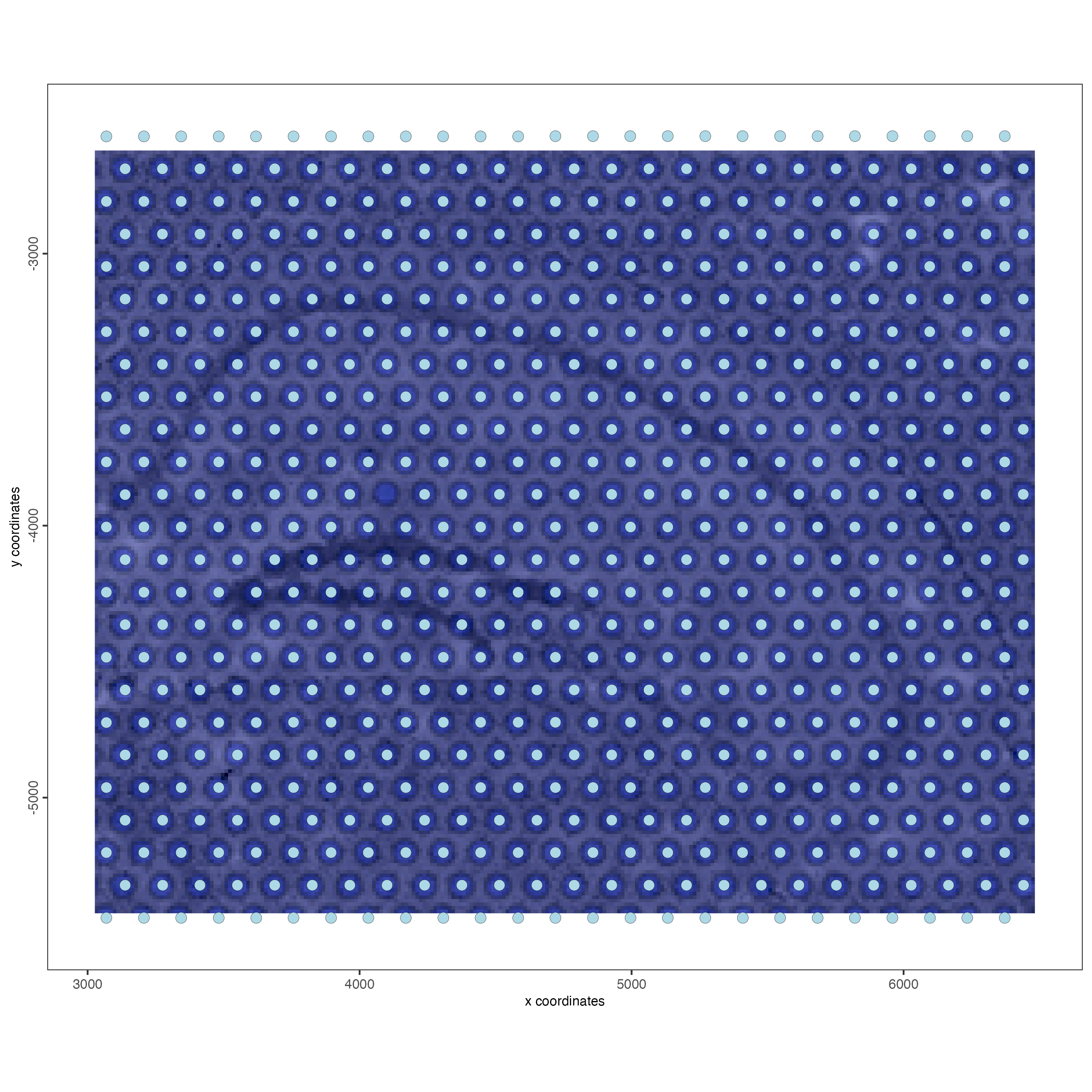
spatPlot2D(gobject = vizgen_object,
           show_image = TRUE)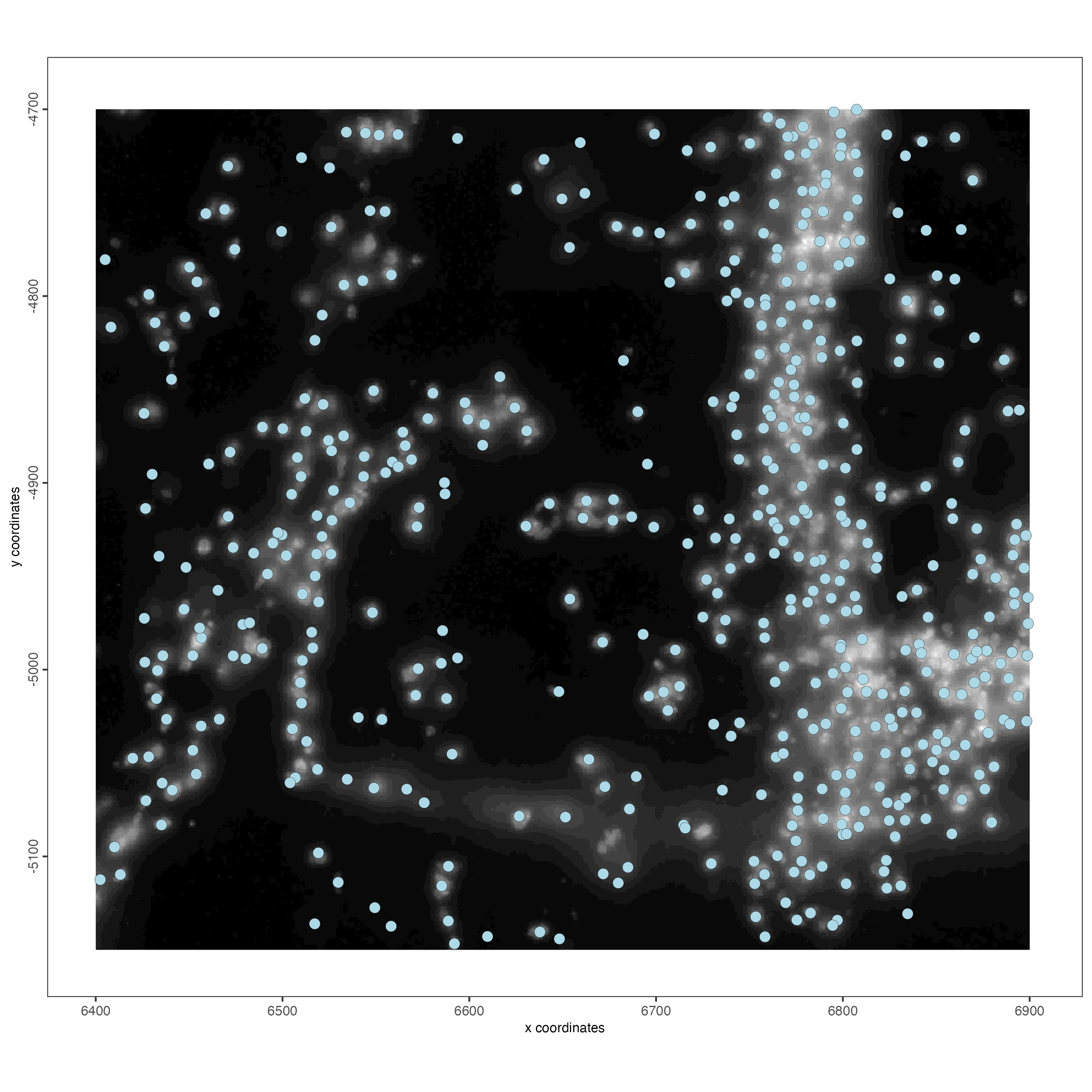
5 Process the object
The function processGiotto performs the filtering,
normalization, statistics and matrix adjustment calculation in a single
step. You can pass the regular arguments from the individual
filterGiotto, normalizeGiotto,
addStatistics, and adjustGiottoMatrix
functions to perform these steps.
visium_object <- processGiotto(visium_object,
                               filter_params = list(expression_threshold = 1,
                                                    feat_det_in_min_cells = 1,
                                                    min_det_feats_per_cell = 50),
                               norm_params = list(scalefactor = 6000),
                               adjust_params = list(covariate_columns = "leiden_clus"))


vizgen_object <- processGiotto(gobject = vizgen_object,
                               filter_params = list(expression_threshold = 1,
                                                    feat_det_in_min_cells = 1,
                                                    min_det_feats_per_cell = 1),
                               adjust_params = NULL)
6 Dimension reduction and Clustering
- UMAP
plotUMAP(gobject = visium_object,
         cell_color = "leiden_clus",
         show_NN_network = TRUE,
         point_size = 2.5)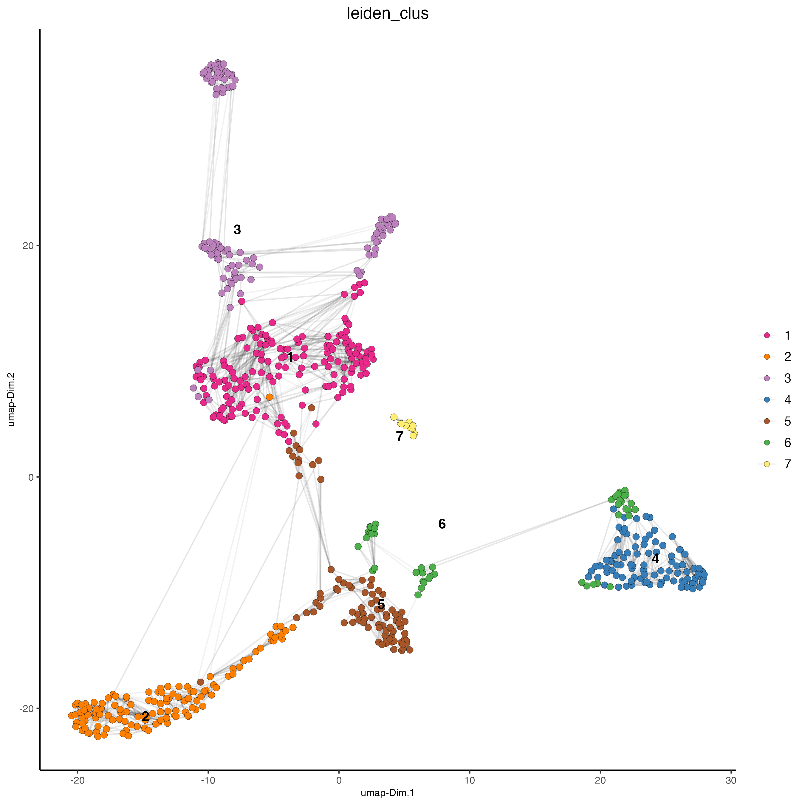
vizgen_object <- runPCA(vizgen_object)

vizgen_object <- runUMAP(vizgen_object)

vizgen_object <- createNearestNetwork(vizgen_object)

vizgen_object <- doLeidenCluster(vizgen_object)

plotUMAP(gobject = vizgen_object,
         cell_color = "leiden_clus",
         show_NN_network = TRUE,
         point_size = 2.5)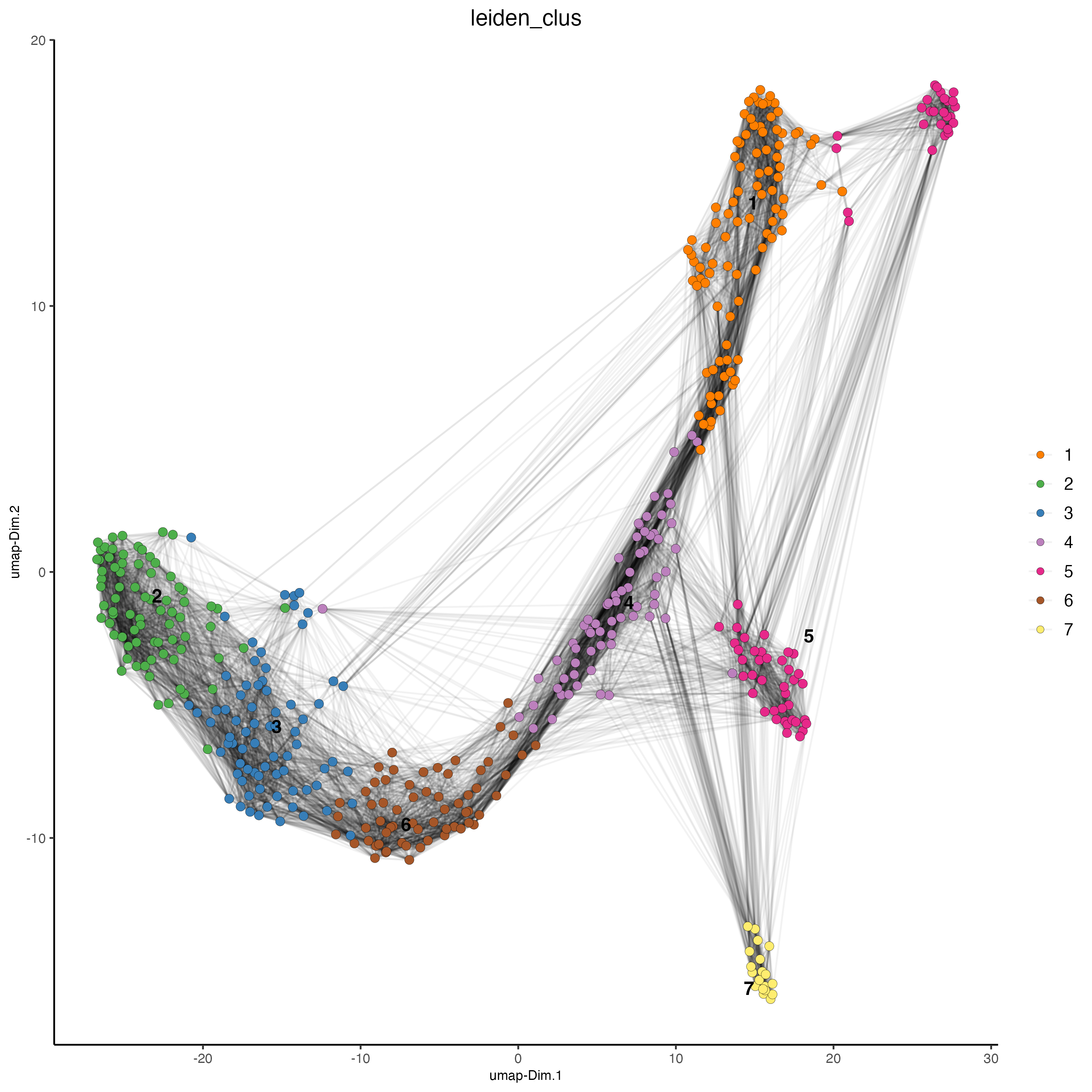
- tSNE
plotTSNE(gobject = visium_object,
         cell_color = "leiden_clus",
         show_NN_network = FALSE,
         point_size = 2.5)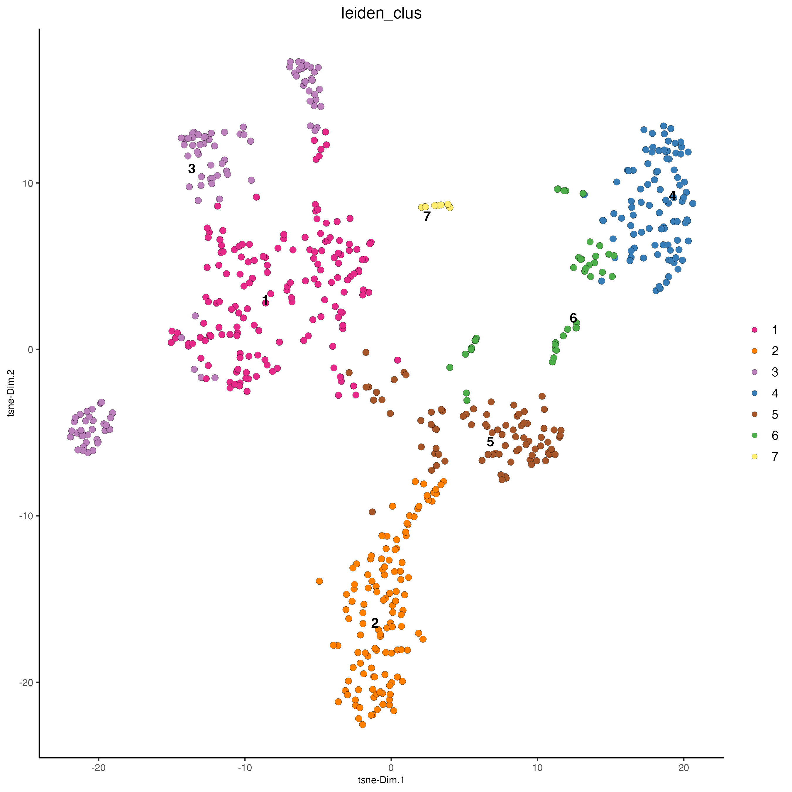
vizgen_object <- runtSNE(vizgen_object)

plotTSNE(gobject = vizgen_object,
         cell_color = "leiden_clus",
         show_NN_network = TRUE,
         point_size = 2.5)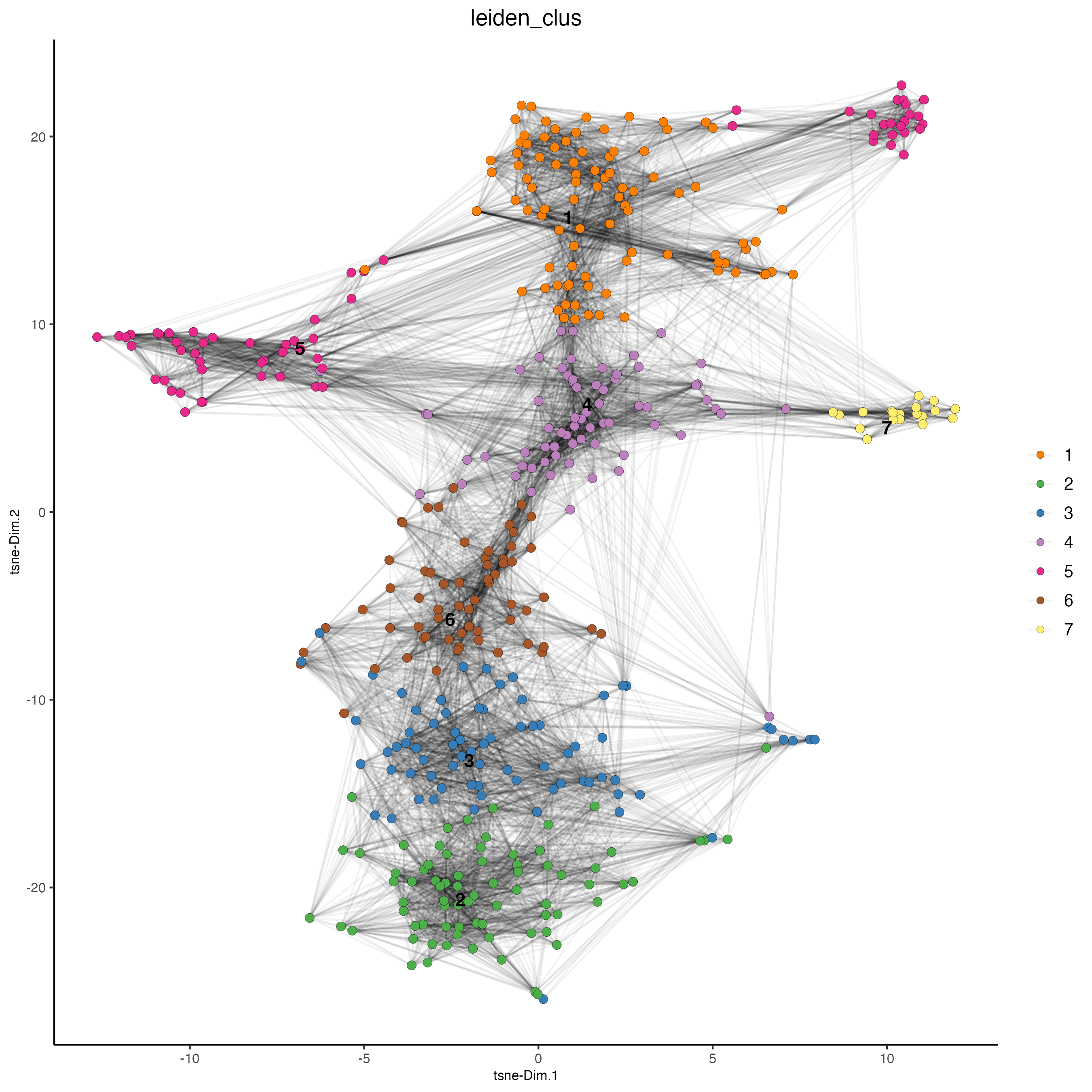
- Spatial plots
spatPlot2D(gobject = visium_object,
           cell_color = "leiden_clus",
           show_image = TRUE,
           point_size = 4)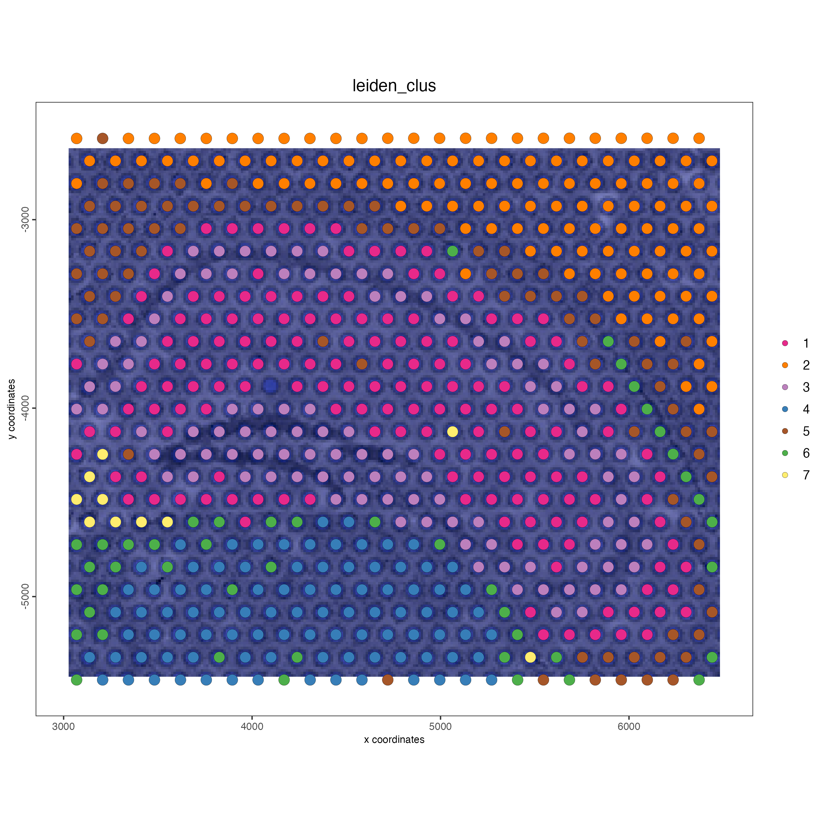
spatPlot2D(gobject = vizgen_object,
           cell_color = "leiden_clus",
           show_image = TRUE,
           point_size = 3)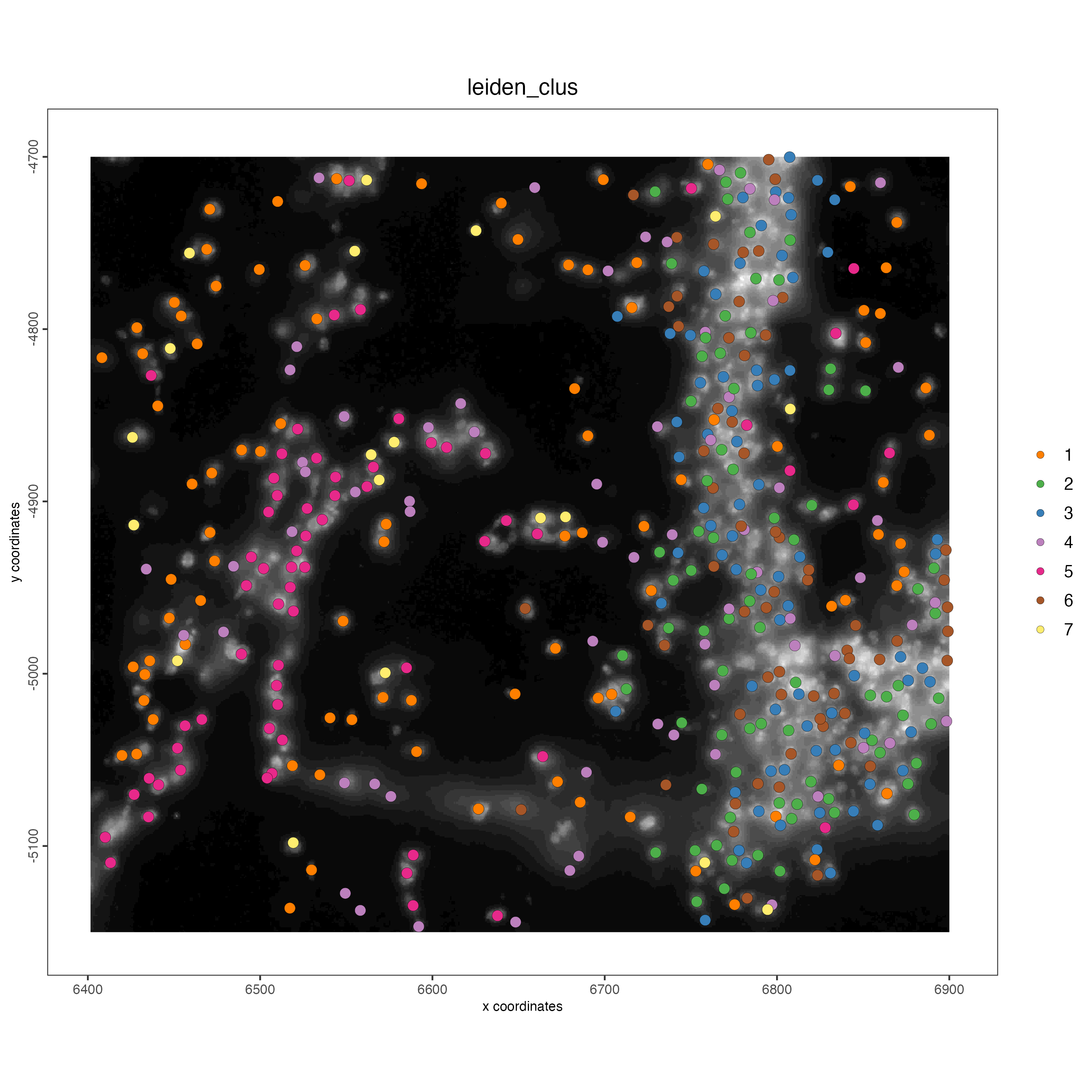
7 Session info
R version 4.4.0 (2024-04-24)
Platform: x86_64-apple-darwin20
Running under: macOS Sonoma 14.6.1

Matrix products: default
BLAS:   /System/Library/Frameworks/Accelerate.framework/Versions/A/Frameworks/vecLib.framework/Versions/A/libBLAS.dylib
LAPACK: /Library/Frameworks/R.framework/Versions/4.4-x86_64/Resources/lib/libRlapack.dylib;  LAPACK version 3.12.0

locale:
[1] en_US.UTF-8/en_US.UTF-8/en_US.UTF-8/C/en_US.UTF-8/en_US.UTF-8

time zone: America/New_York
tzcode source: internal

attached base packages:
[1] stats     graphics  grDevices utils     datasets  methods   base

other attached packages:
[1] Giotto_4.1.1      GiottoClass_0.3.5

loaded via a namespace (and not attached):
  [1] colorRamp2_0.1.0            deldir_2.0-4                rlang_1.1.4
  [4] magrittr_2.0.3              GiottoUtils_0.1.11          matrixStats_1.3.0
  [7] compiler_4.4.0              png_0.1-8                   systemfonts_1.1.0
 [10] vctrs_0.6.5                 reshape2_1.4.4              stringr_1.5.1
 [13] pkgconfig_2.0.3             SpatialExperiment_1.14.0    crayon_1.5.3
 [16] fastmap_1.2.0               backports_1.5.0             magick_2.8.4
 [19] XVector_0.44.0              labeling_0.4.3              utf8_1.2.4
 [22] rmarkdown_2.28              UCSC.utils_1.0.0            ragg_1.3.2
 [25] purrr_1.0.2                 xfun_0.47                   beachmat_2.20.0
 [28] zlibbioc_1.50.0             GenomeInfoDb_1.40.1         jsonlite_1.8.8
 [31] DelayedArray_0.30.1         BiocParallel_1.38.0         terra_1.7-78
 [34] irlba_2.3.5.1               parallel_4.4.0              R6_2.5.1
 [37] stringi_1.8.4               RColorBrewer_1.1-3          limma_3.60.4
 [40] reticulate_1.38.0           GenomicRanges_1.56.1        scattermore_1.2
 [43] Rcpp_1.0.13                 SummarizedExperiment_1.34.0 knitr_1.48
 [46] R.utils_2.12.3              FNN_1.1.4                   IRanges_2.38.1
 [49] Matrix_1.7-0                igraph_2.0.3                tidyselect_1.2.1
 [52] rstudioapi_0.16.0           abind_1.4-5                 yaml_2.3.10
 [55] codetools_0.2-20            lattice_0.22-6              tibble_3.2.1
 [58] plyr_1.8.9                  Biobase_2.64.0              withr_3.0.1
 [61] Rtsne_0.17                  evaluate_0.24.0             pillar_1.9.0
 [64] MatrixGenerics_1.16.0       checkmate_2.3.2             stats4_4.4.0
 [67] plotly_4.10.4               generics_0.1.3              dbscan_1.2-0
 [70] sp_2.1-4                    S4Vectors_0.42.1            ggplot2_3.5.1
 [73] munsell_0.5.1               scales_1.3.0                GiottoData_0.2.13
 [76] gtools_3.9.5                glue_1.7.0                  lazyeval_0.2.2
 [79] tools_4.4.0                 GiottoVisuals_0.2.5         data.table_1.16.0
 [82] ScaledMatrix_1.12.0         cowplot_1.1.3               grid_4.4.0
 [85] tidyr_1.3.1                 colorspace_2.1-1            SingleCellExperiment_1.26.0
 [88] GenomeInfoDbData_1.2.12     BiocSingular_1.20.0         rsvd_1.0.5
 [91] cli_3.6.3                   textshaping_0.4.0           fansi_1.0.6
 [94] S4Arrays_1.4.1              viridisLite_0.4.2           dplyr_1.1.4
 [97] uwot_0.2.2                  gtable_0.3.5                R.methodsS3_1.8.2
[100] digest_0.6.37               BiocGenerics_0.50.0         SparseArray_1.4.8
[103] ggrepel_0.9.5               rjson_0.2.22                htmlwidgets_1.6.4
[106] farver_2.1.2                htmltools_0.5.8.1           R.oo_1.26.0
[109] lifecycle_1.0.4             httr_1.4.7                  statmod_1.5.0