1 Dataset explanation
10X genomics launched a platform to obtain spatial expression data using a Visium Spatial Gene Expression slide.
Visium allows you to perform spatial transcriptomics, which combines histological information with whole transcriptome gene expression profiles (fresh frozen or FFPE) to provide you with spatially resolved gene expression.
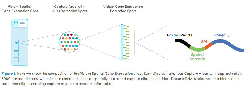
You can use standard fixation and staining techniques, including hematoxylin and eosin (H&E) staining, to visualize tissue sections on slides using a brightfield microscope and immunofluorescence (IF) staining to visualize protein detection in tissue sections on slides using a fluorescent microscope.
High resolution png from original tissue:
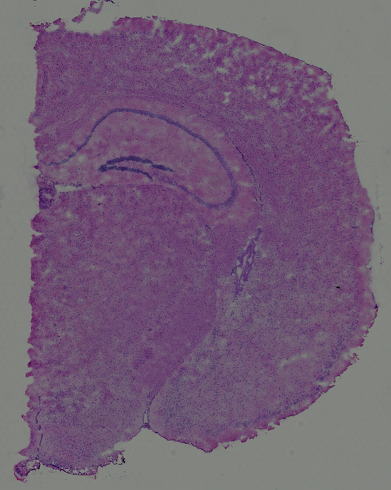
The visium fresh frozen mouse brain tissue (Strain C57BL/6) dataset was obtained from 10X genomics. The tissue was embedded and cryosectioned as described in Visium Spatial Protocols - Tissue Preparation Guide (Demonstrated Protocol CG000240). Tissue sections of 10 µm thickness from a slice of the coronal plane were placed on Visium Gene Expression Slides.
You can find more information about this sample here
2 Download dataset
You need to download the expression matrix and spatial information by running these commands:
dir.create("/path/to/data/")

download.file(url = "https://cf.10xgenomics.com/samples/spatial-exp/1.1.0/V1_Adult_Mouse_Brain/V1_Adult_Mouse_Brain_raw_feature_bc_matrix.tar.gz",
              destfile = "data/V1_Adult_Mouse_Brain_raw_feature_bc_matrix.tar.gz")

download.file(url = "https://cf.10xgenomics.com/samples/spatial-exp/1.1.0/V1_Adult_Mouse_Brain/V1_Adult_Mouse_Brain_spatial.tar.gz",
              destfile = "data/V1_Adult_Mouse_Brain_spatial.tar.gz")
After downloading, unzip the gz files. You should get the “raw_feature_bc_matrix” and “spatial” folders inside your “/path/to/data/”.
3 Set up Giotto environment
Ensure that the Giotto package is installed. Additionally, check that the mini conda Giotto environment with Python dependencies is installed.
If you have installation troubles, visit the Installation and Frequently Asked Questions sections.
# Ensure Giotto Suite is installed.
if(!"Giotto" %in% installed.packages()) {
  pak::pkg_install("drieslab/Giotto")
}

# Ensure the Python environment for Giotto has been installed.
genv_exists <- Giotto::checkGiottoEnvironment()
if(!genv_exists){
  # The following command need only be run once to install the Giotto environment.
  Giotto::installGiottoEnvironment()
}
4 Set the Giotto instructions
{Giotto} instructions are used to apply settings to giotto object behavior at the project level. Each giotto object needs a set of instructions information that can either be manually set or generated with defaults when the giotto object is first created. Once added, these instructions are stored in the giotto object @instructions slot.
library(Giotto)

# Set the results directory to save plots
results_folder <- "path/to/results"

# Optional: Specify the path to a Python executable within a conda or miniconda
# environment. If set to NULL (default), the Python executable within the previously installed Giotto environment will be used.
python_path <- NULL # alternatively, "/local/python/path/python" if desired.

# Create Giotto Instructions
instructions <- createGiottoInstructions(save_dir = results_folder,
                                         save_plot = TRUE,
                                         show_plot = FALSE,
                                         return_plot = FALSE,
                                         python_path = python_path)
5 Create the Giotto bject and visualize
createGiottoVisiumObject() will look for the standardized files organization from the Visium technology in the data folder and will automatically load the expression and spatial information to create the Giotto object.
## provide path to visium folder
data_path <- "/path/to/data/"

## read the data
visium_brain <- createGiottoVisiumObject(visium_dir = data_path,
                                         expr_data = "raw",
                                         png_name = "tissue_lowres_image.png",
                                         gene_column_index = 2,
                                         instructions = instructions)

## show associated images with giotto object
showGiottoImageNames(visium_brain) # "image" is the default name

## check metadata
pDataDT(visium_brain)
6 Subset on spots that were covered by tissue
Use the metadata column “in_tissue” to highlight the spots corresponding to the tissue area.
spatPlot2D(gobject = visium_brain,
           cell_color = "in_tissue",
           point_size = 3,
           cell_color_code = c("0" = "lightgrey", "1" = "blue"),
           show_image = TRUE,
           image_name = "image")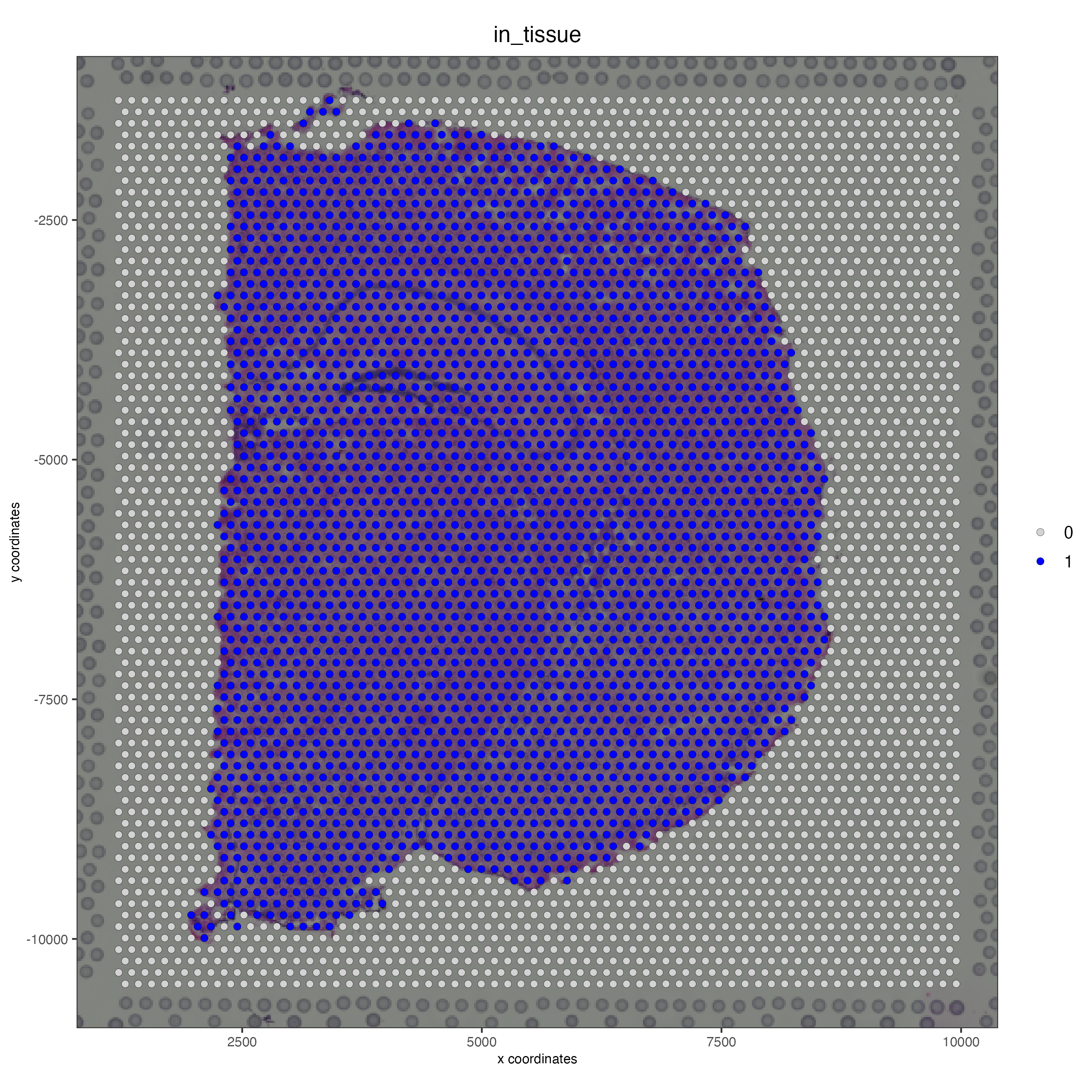
Use the same metadata column “in_tissue” to subset the object and keep only the spots corresponding to the tissue area.
metadata <- pDataDT(visium_brain)
in_tissue_barcodes <- metadata[in_tissue == 1]$cell_ID

visium_brain <- subsetGiotto(visium_brain,
                             cell_ids = in_tissue_barcodes)
7 Quality control
Use the function addStatistics() to count the number of features per spot. The statistics information will be stored in the metadata table under the new column “nr_feats”. Then, use this column to visualize the number of features per spot across the sample.
visium_brain_statistics <- addStatistics(gobject = visium_brain,
                                         expression_values = "raw")

## visualize
spatPlot2D(gobject = visium_brain_statistics,
           cell_color = "nr_feats",
           color_as_factor = FALSE)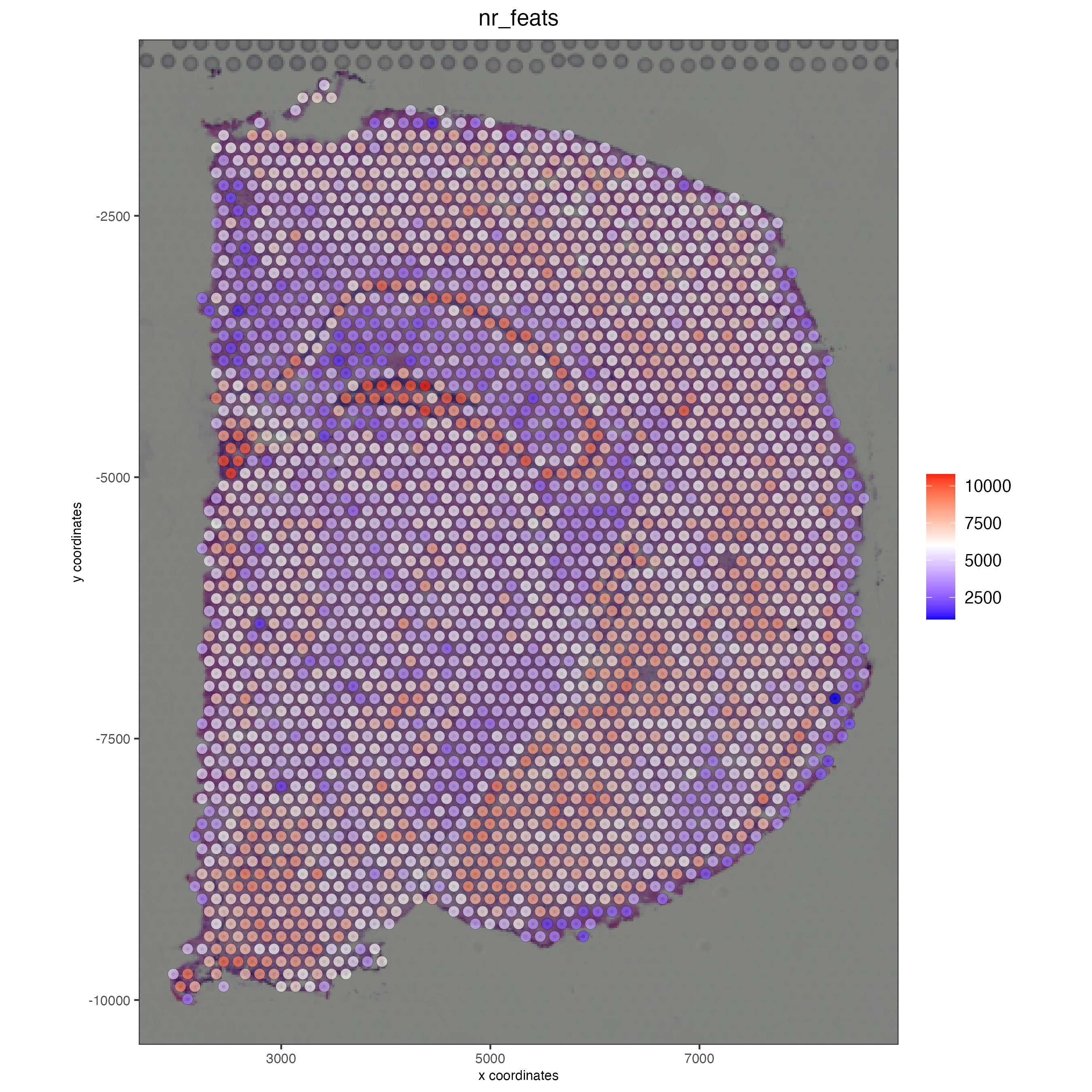
filterDistributions() creates a histogram to show the distribution of features per spot across the sample.
filterDistributions(gobject = visium_brain_statistics,
                    detection = "cells")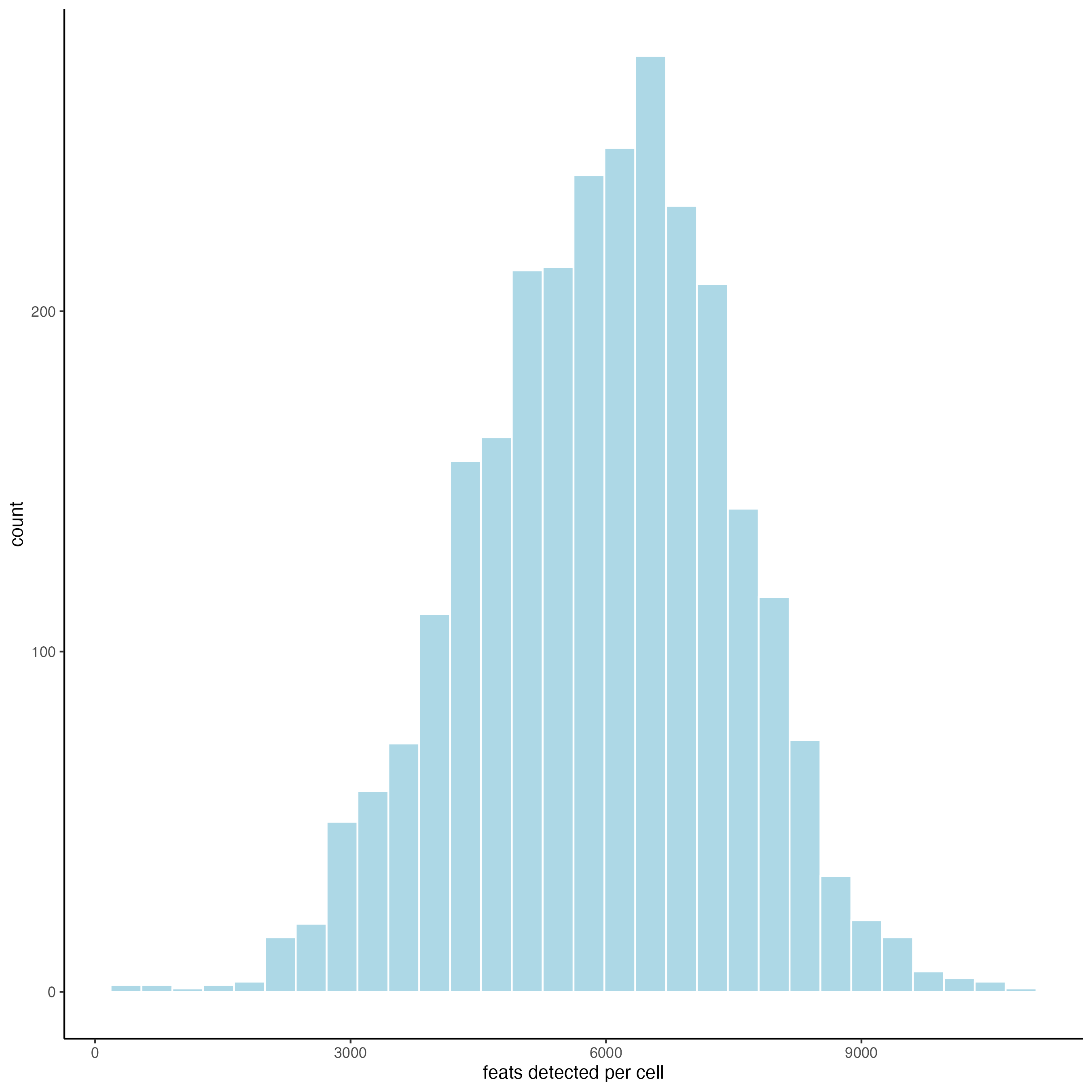
When setting the detection = “feats”, the histogram shows the distribution of spots with certain number of features across the sample.
filterDistributions(gobject = visium_brain_statistics,
                    detection = "feats")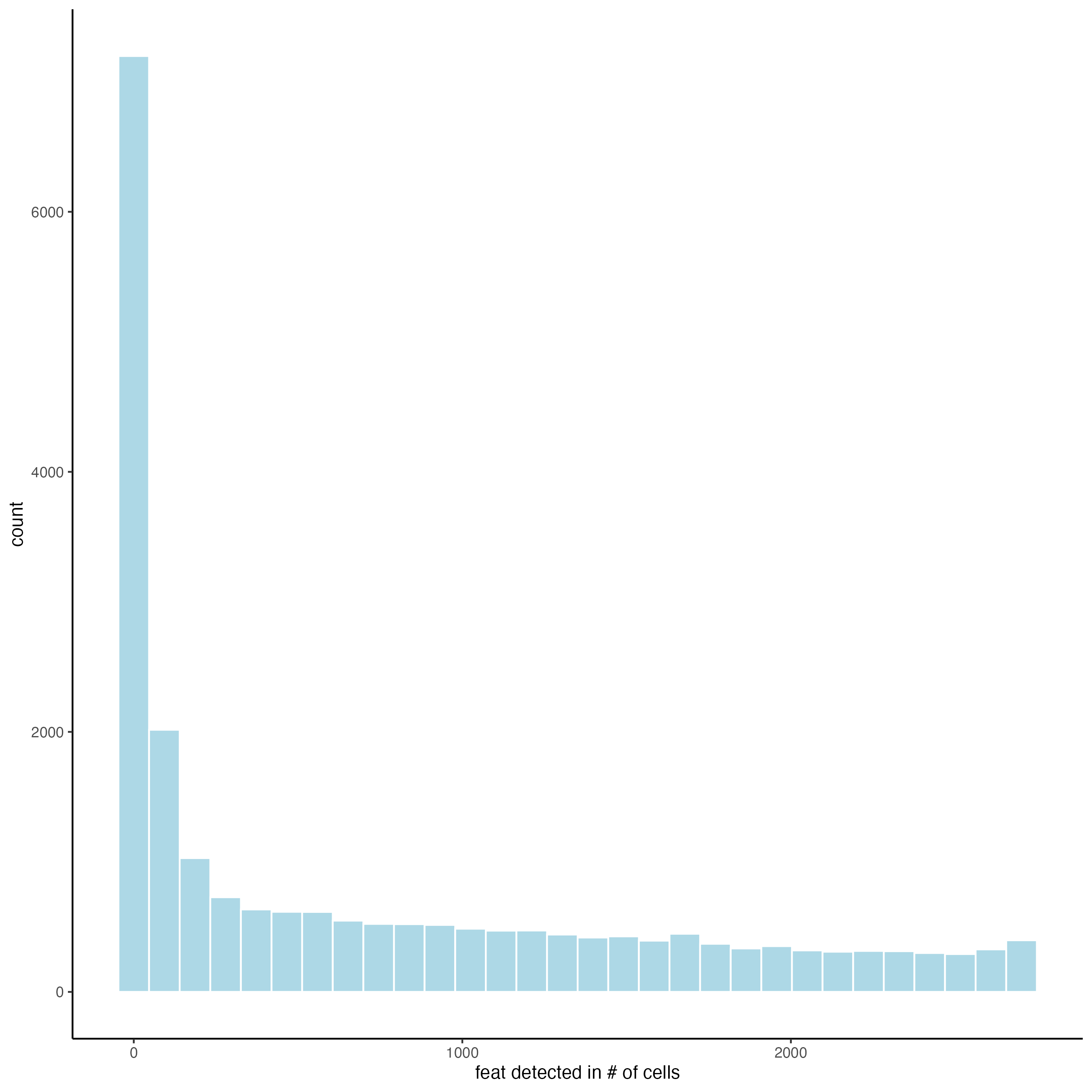
filterCombinations() may be used to test how different filtering parameters will affect the number of cells and features in the filtered data:
filterCombinations(gobject = visium_brain_statistics,
                   expression_thresholds = c(1, 2, 3),
                   feat_det_in_min_cells = c(50, 100, 200),
                   min_det_feats_per_cell = c(500, 1000, 1500))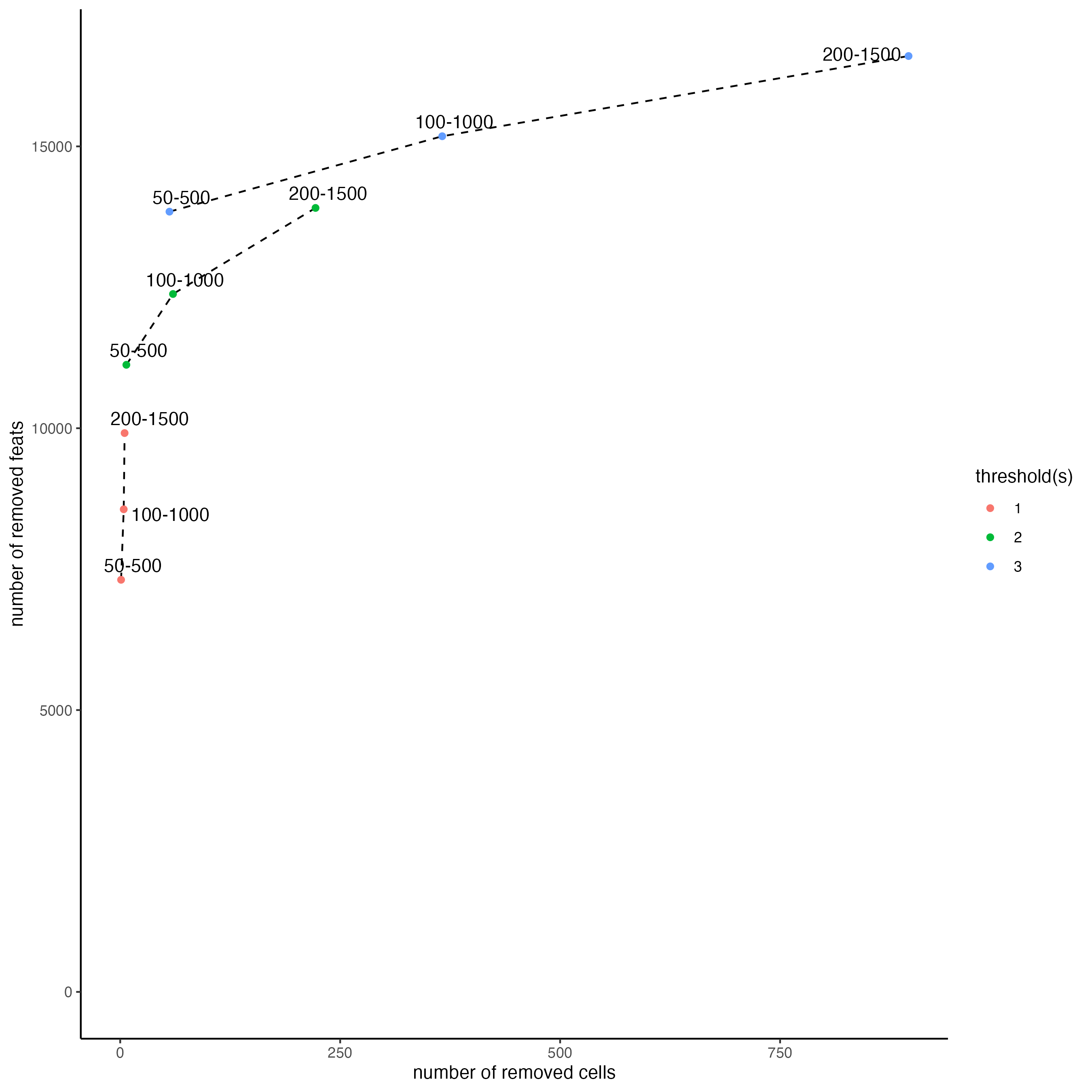
8 Filtering
Use the arguments feat_det_in_min_cells and min_det_feats_per_cell to set the minimal number of cells where an individual feature must be detected and the minimal number of features per spot/cell, respectively, to filter the giotto object. All the features and spots/cells under those thresholds will be removed from the sample.
visium_brain <- filterGiotto(gobject = visium_brain,
                             expression_threshold = 1,
                             feat_det_in_min_cells = 50,
                             min_det_feats_per_cell = 1000,
                             expression_values = "raw",
                             verbose = TRUE)
9 Normalization
Use scalefactor to set the scale factor to use after library size normalization. The default value is 6000, but you can use a different one.
visium_brain <- normalizeGiotto(gobject = visium_brain,
                                scalefactor = 6000,
                                verbose = TRUE)
Calculate the normalized number of features per spot and save the statistics in the metadata table.
visium_brain <- addStatistics(gobject = visium_brain)

## visualize
spatPlot2D(gobject = visium_brain,
           show_image = TRUE,
           point_alpha = 0.7,
           cell_color = "nr_feats",
           color_as_factor = FALSE)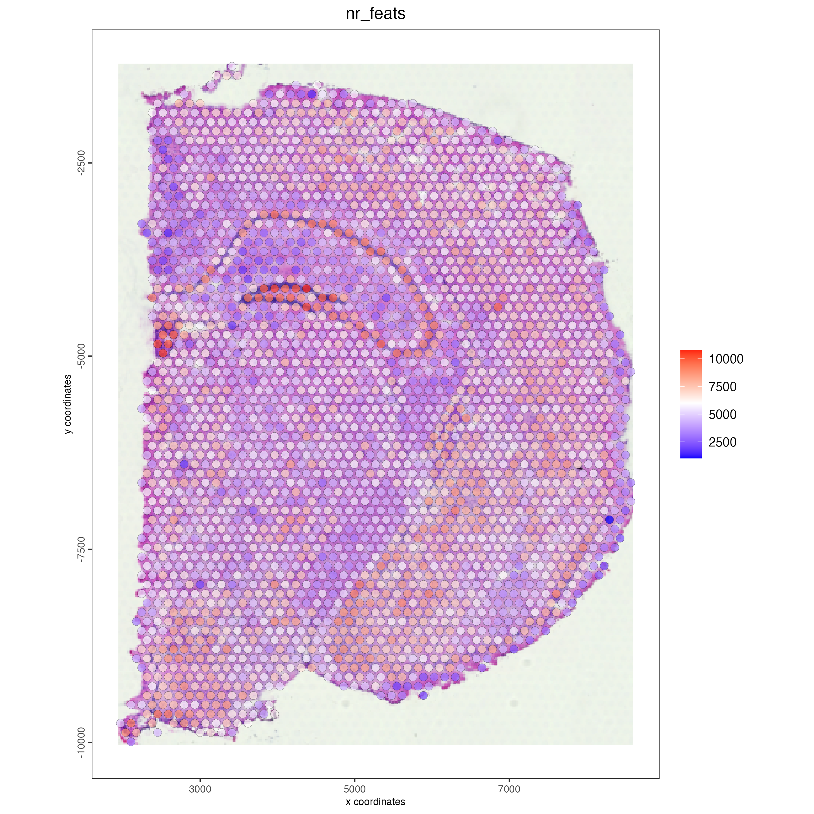
10 Feature selection
Calculating Highly Variable Features (HVF) is necessary to identify genes (or features) that display significant variability across the spots. There are a few methods to choose from depending on the underlying distribution of the data:
- loess regression is used when the relationship between mean expression and variance is non-linear or can be described by a non-parametric model.
visium_brain <- calculateHVF(gobject = visium_brain,
                             method = "cov_loess",
                             save_plot = TRUE)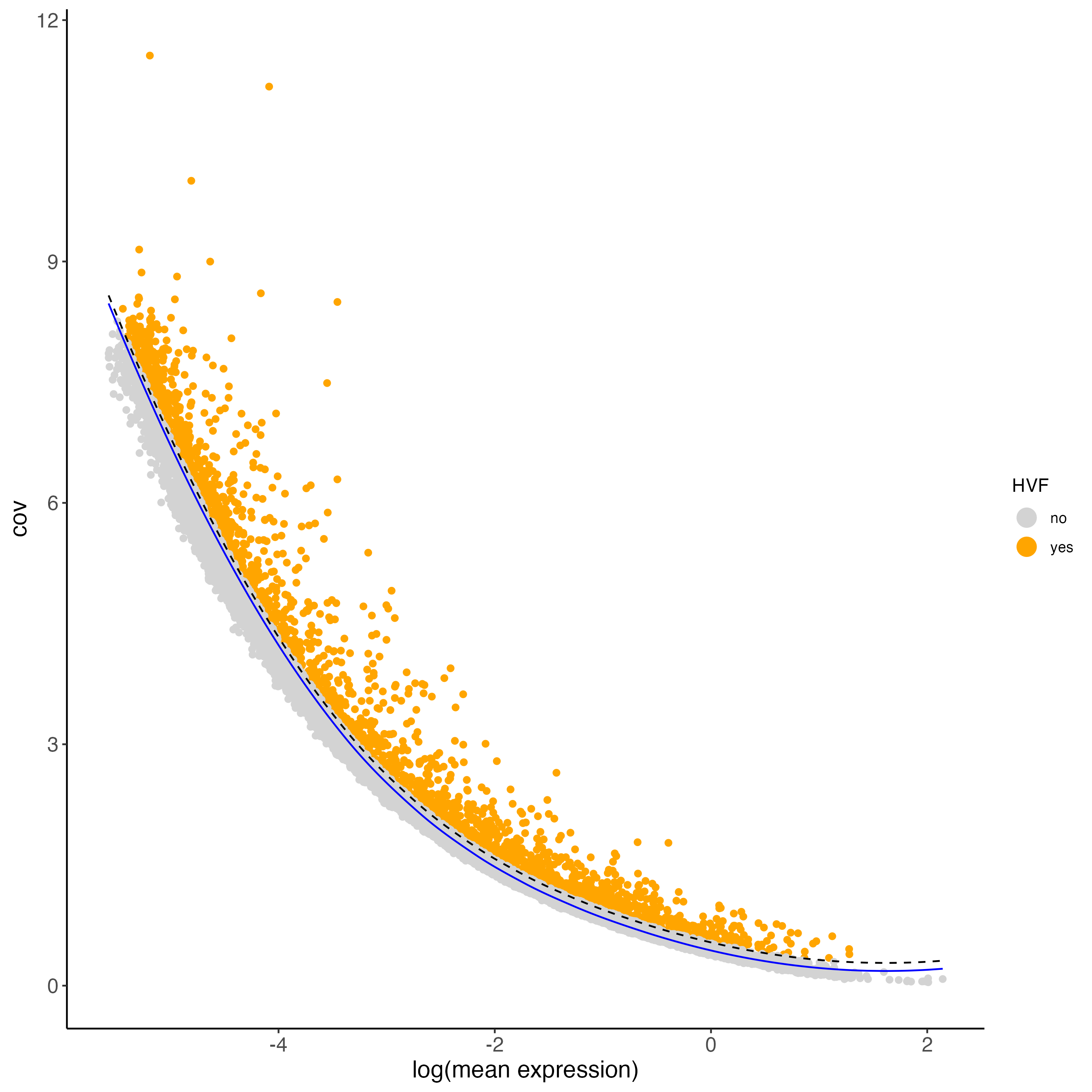
- pearson residuals are used for variance stabilization (to account for technical noise) and highlighting overdispersed genes.
visium_brain <- calculateHVF(gobject = visium_brain,
                             method = "var_p_resid",
                             save_plot = TRUE)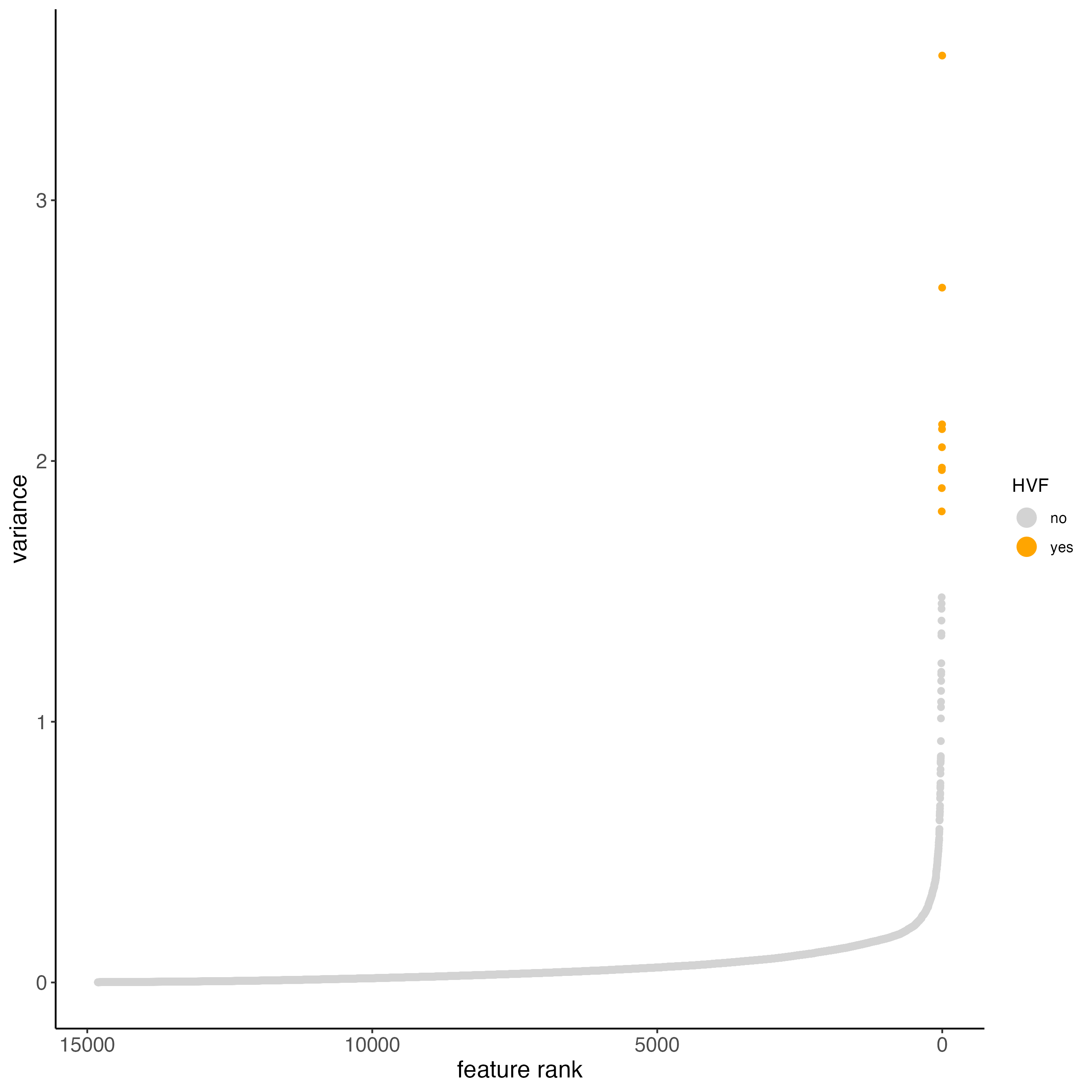
- binned (covariance groups) are used when gene expression variability differs across expression levels or spatial regions, without assuming a specific relationship between mean expression and variance. This is the default method in the calculateHVF() function.
visium_brain <- calculateHVF(gobject = visium_brain,
                             method = "cov_groups",
                             save_plot = TRUE)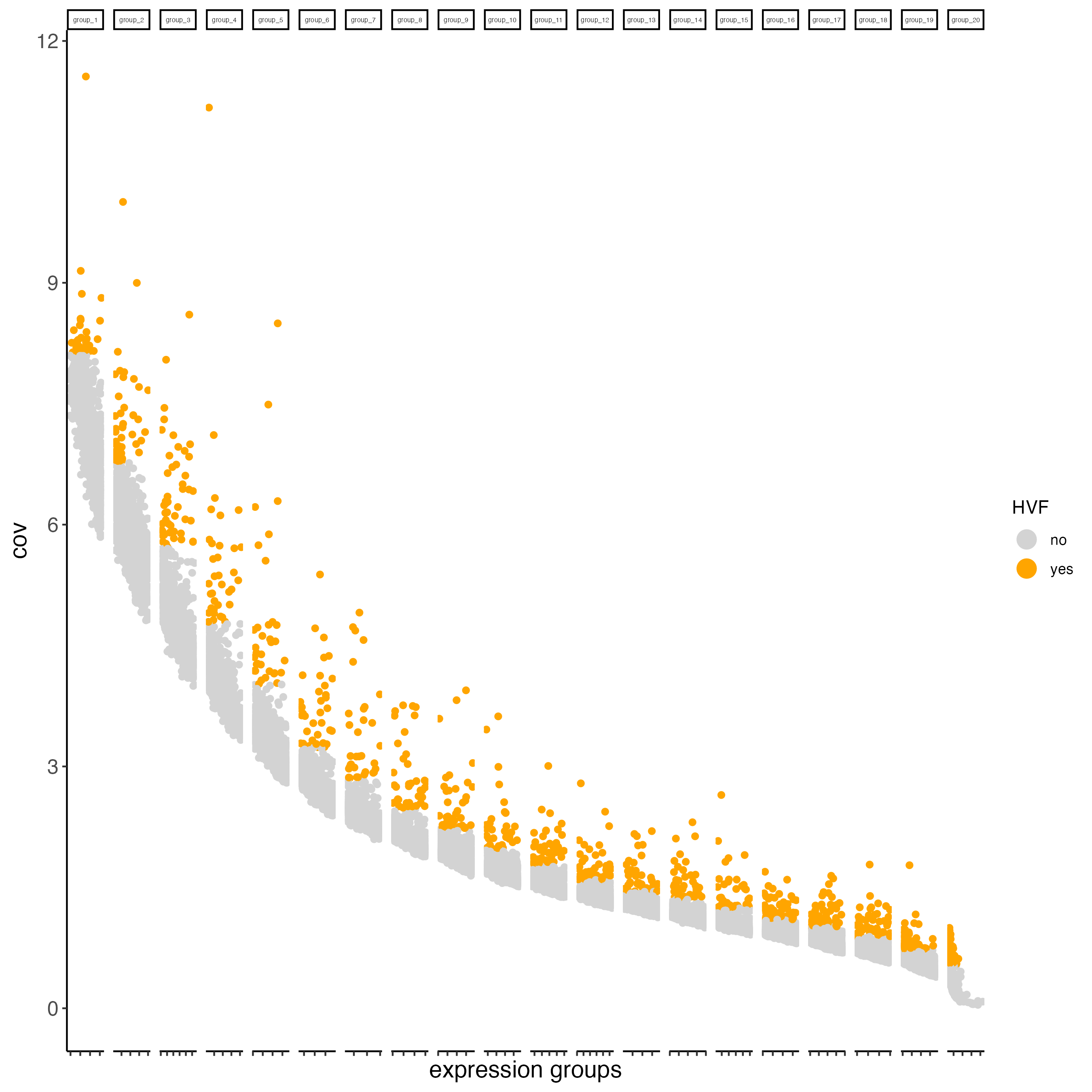
11 Dimension reduction
11.1 PCA
Principal Components Analysis (PCA) is applied to reduce the dimensionality of gene expression data by transforming it into principal components, which are linear combinations of genes ranked by the variance they explain, with the first components capturing the most variance.
- runPCA() will look for the previous calculation of highly variable features, stored as a column in the feature metadata. If the HVF labels are not found in the giotto object, then runPCA() will use all the features available in the sample to calculate the Principal Components.
visium_brain <- runPCA(gobject = visium_brain)- You can also use specific features for the Principal Components calculation, by passing a vector of features in the “feats_to_use” argument.
my_features <- head(getFeatureMetadata(visium_brain,
                                       output = "data.table")$feat_ID,
                    1000)

visium_brain <- runPCA(gobject = visium_brain,
                       feats_to_use = my_features,
                       name = "custom_pca")
Create a screeplot to visualize the percentage of variance explained by each component.
screePlot(gobject = visium_brain,
          ncp = 30)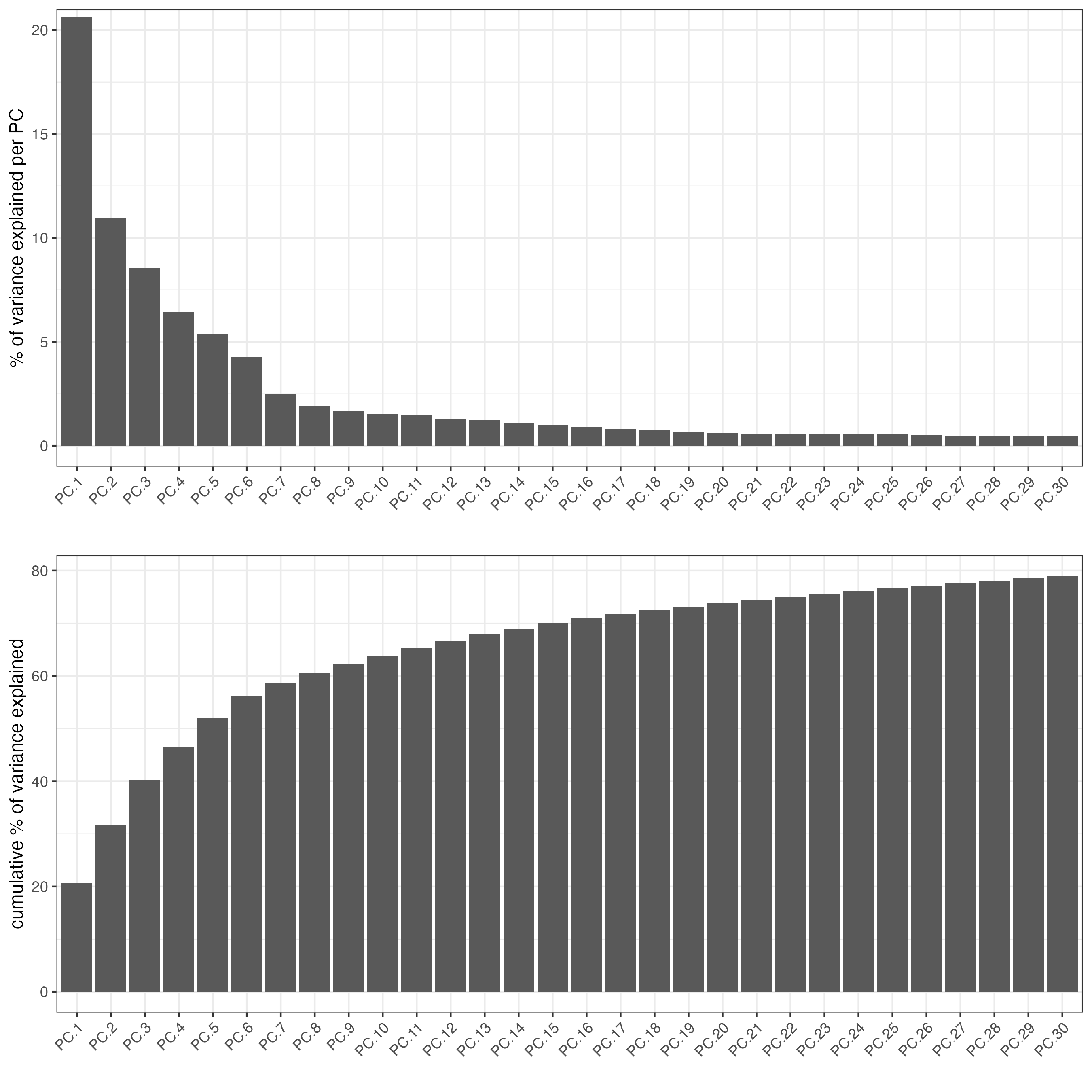
- Visualize the PCA calculated using the HVFs.
plotPCA(gobject = visium_brain)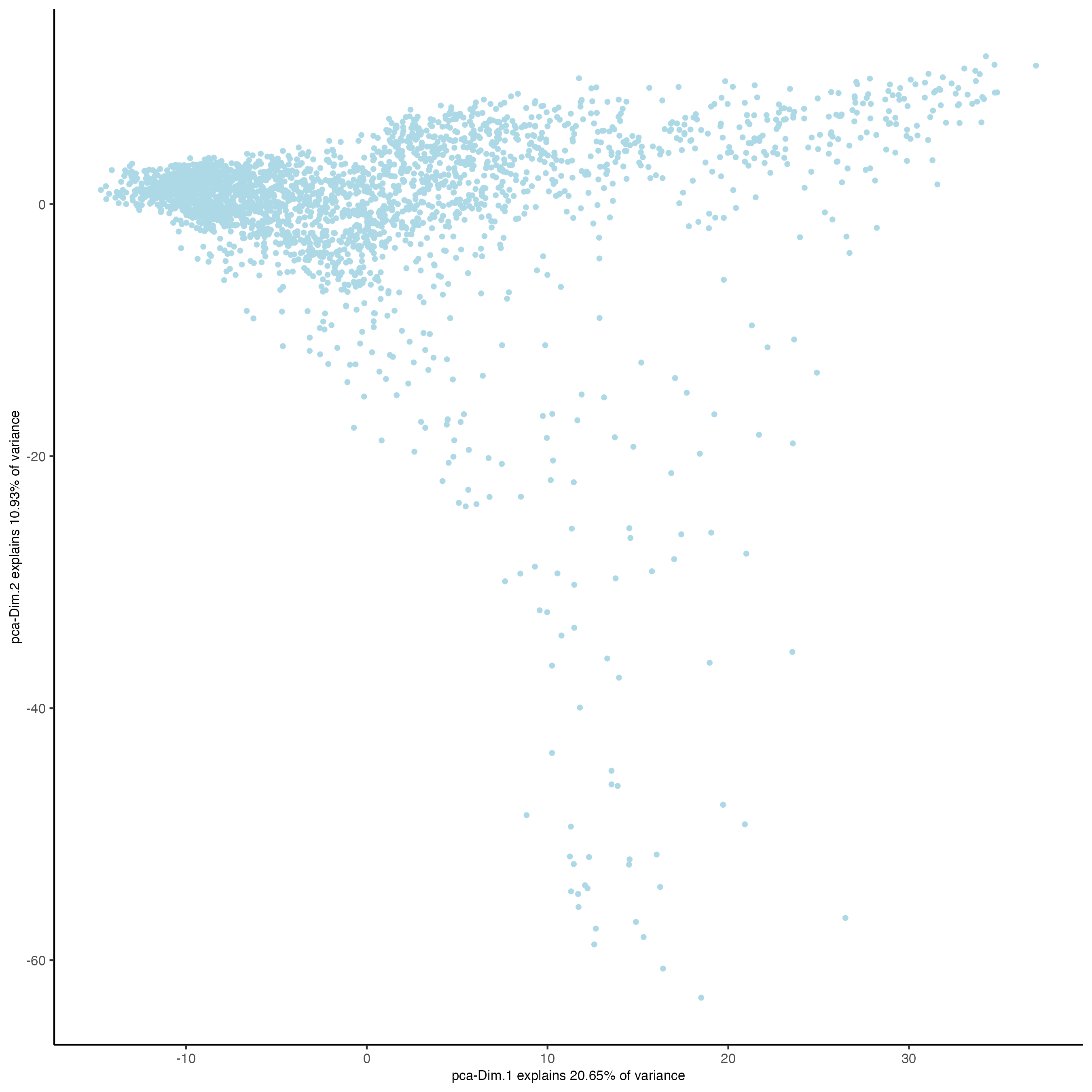
- Visualize the custom PCA calculated using the vector of features.
plotPCA(gobject = visium_brain,
        dim_reduction_name = "custom_pca")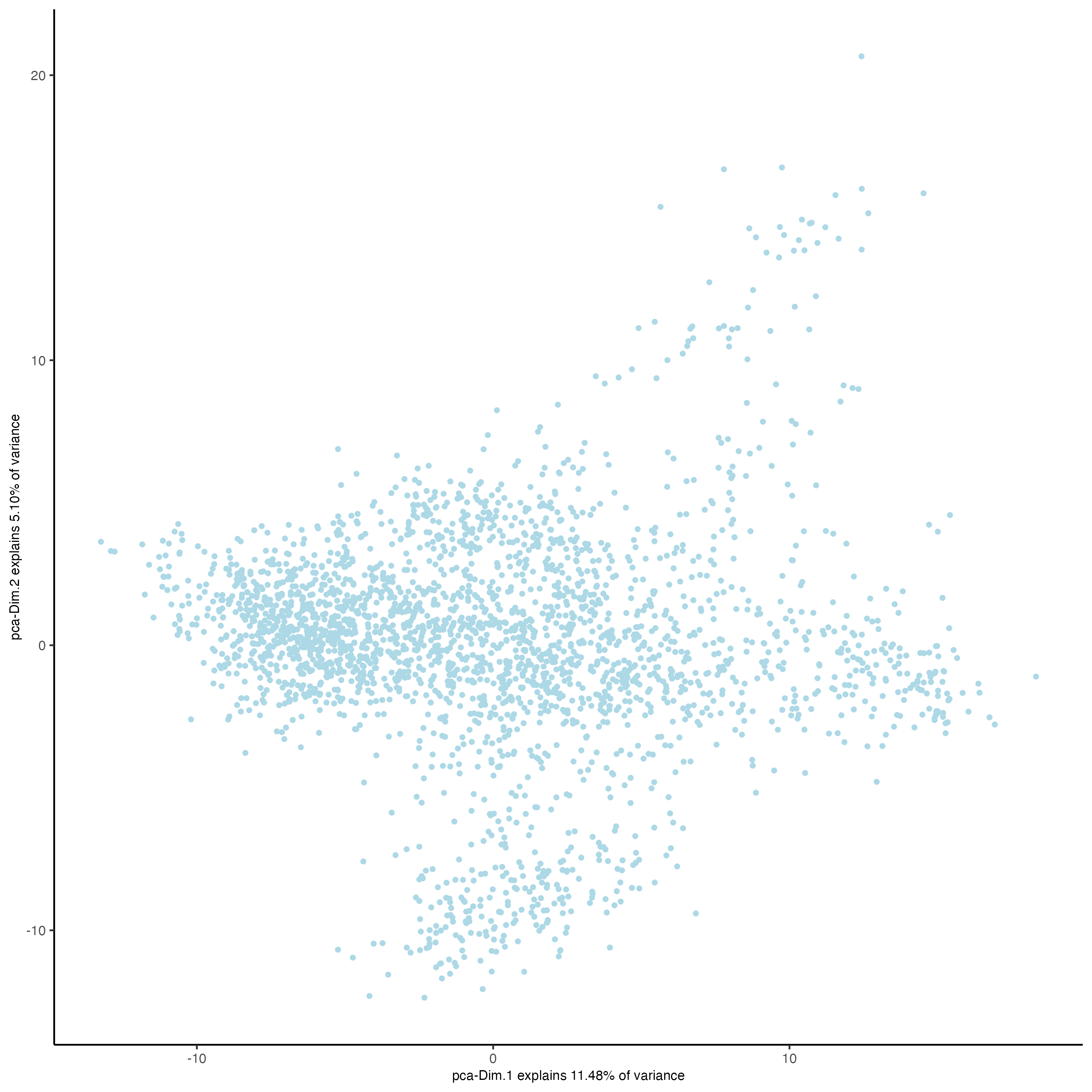
11.2 UMAP
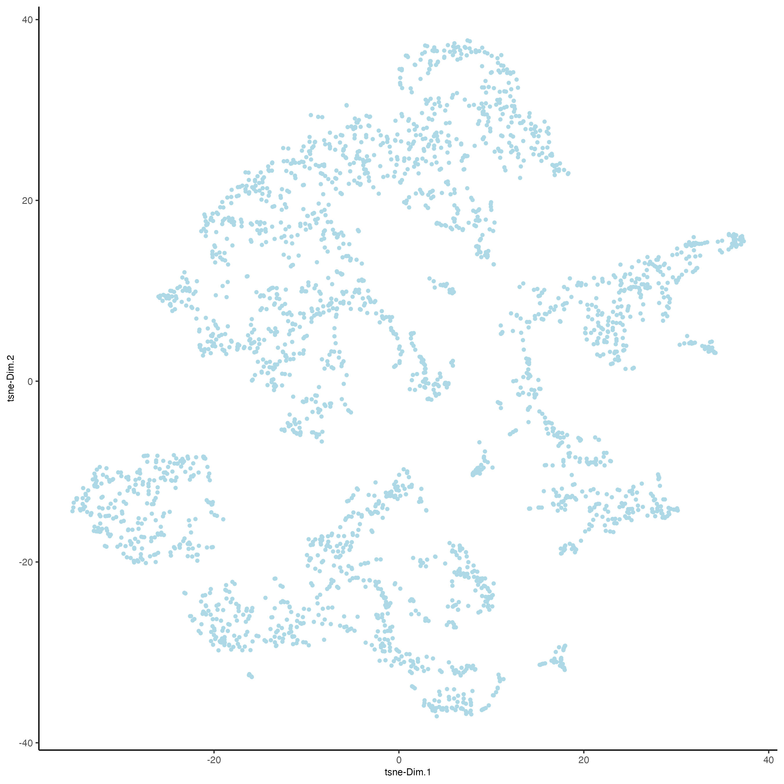
Unlike PCA, Uniform Manifold Approximation and Projection (UMAP) and t-Stochastic Neighbor Embedding (t-SNE) do not assume linearity. After running PCA, UMAP or t-SNE allows you to visualize the dataset in 2D.
## run UMAP on PCA space (default)
visium_brain <- runUMAP(visium_brain,
                        dimensions_to_use = 1:10)

plotUMAP(gobject = visium_brain)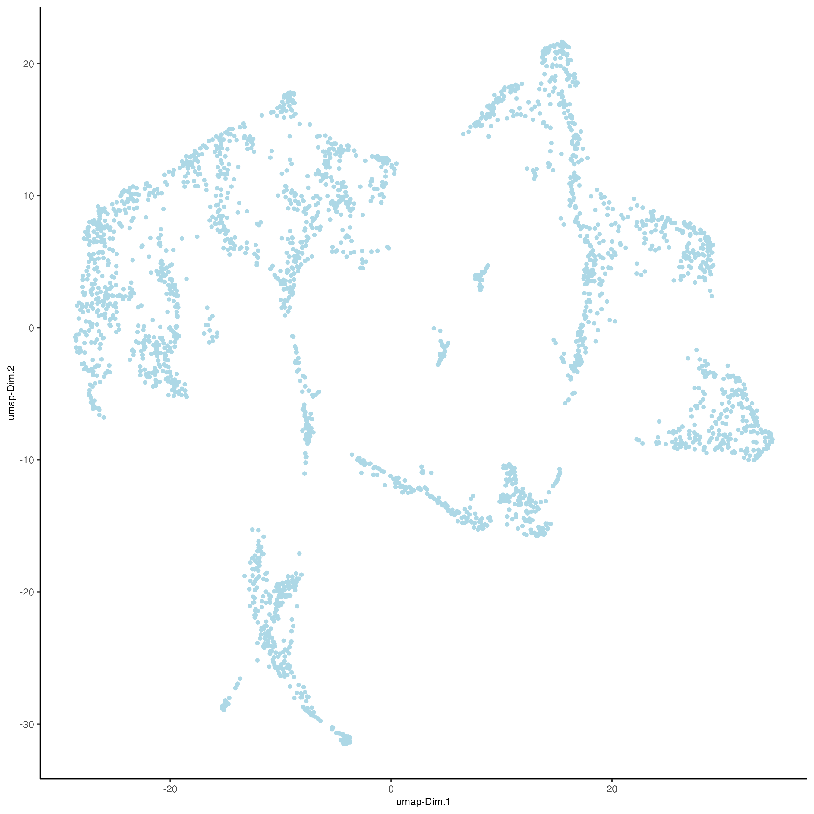
12 Clustering
12.1 Calculate the nearest neighbors
In preparation for the clustering calculation, finding the spots/cells with similar expression patterns is needed. There are two methods available in Giotto:
- Create a sNN network (default)
The shared Nearest Neighbor algorithm defines the similarity between a pair of points in terms of their shared nearest neighbors. That is, the similarity between two points is “confirmed” by their common (shared) near neighbors. If point A is close to point B and if they are both close to a set of points C then we can say that A and B are close with greater confidence since their similarity is “confirmed” by the points in set C. You can find more information about this method here. By default, createNearestNetwork() calculates 30 shared Nearest Neighbors for each spot/cell, but you can modify this number using the “k” parameter.
visium_brain <- createNearestNetwork(gobject = visium_brain,
                                     dimensions_to_use = 1:10,
k = 15)- Create a kNN network
The K-Nearest Neighbors (kNN) algorithm operates on the principle of likelihood of similarity. It posits that similar data points tend to cluster near each other in space. You can find more information about this method here. By default, createNearestNetwork() finds the 30 K-Nearest Neighbors to each spot/cell, but you can modify this number using the “k” parameter.
visium_brain <- createNearestNetwork(gobject = visium_brain,
                                     dimensions_to_use = 1:10,
                                     k = 15,
                                     type = "kNN")
12.2 Leiden clustering
This algorithm is more complicated than the Louvain algorithm and have an accurate and fast result for the computation time. The Leiden algorithm consists of three phases. The first phase is the modularity optimization process, the second phase is the refinement of partition, and the third phase is the community aggregation process. This algorithm performs well on small, medium and large-scale networks. You can find more information about Louvain and Leiden clustering here
- Run the Leiden clustering algorithm.
visium_brain <- doLeidenCluster(gobject = visium_brain,
                                resolution = 0.4,
n_iterations = 1000)- Plot dimension and spatial plots using the Leiden clusters information.
plotPCA(gobject = visium_brain,
        cell_color = "leiden_clus")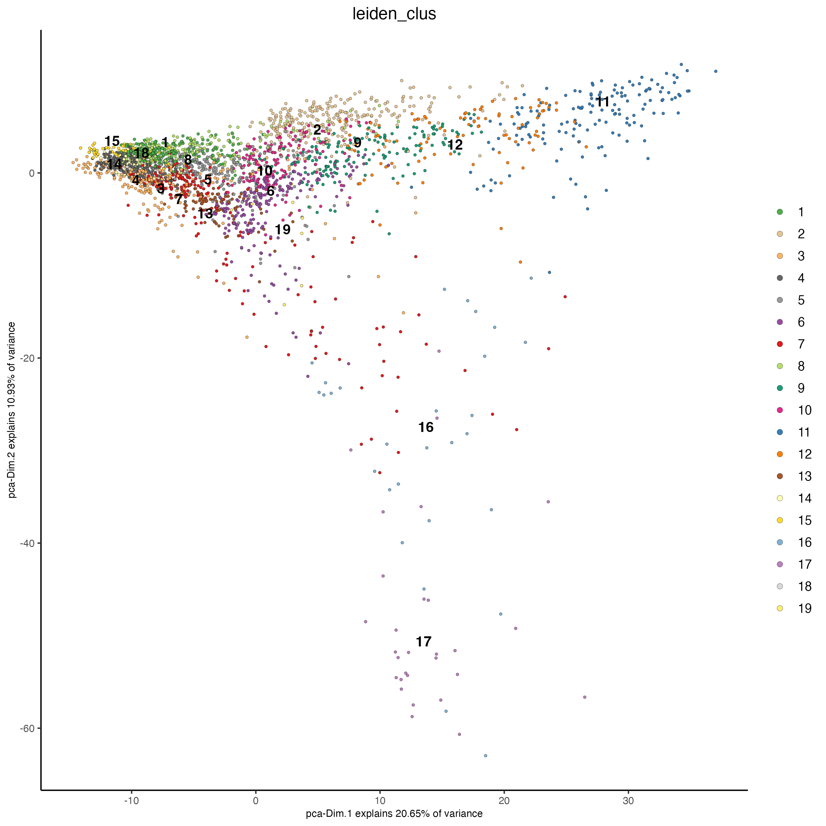
Set the argument “show_NN_network = TRUE” to visualize the connections between spots.
plotUMAP(gobject = visium_brain,
         cell_color = "leiden_clus",
         show_NN_network = TRUE,
         point_size = 2.5)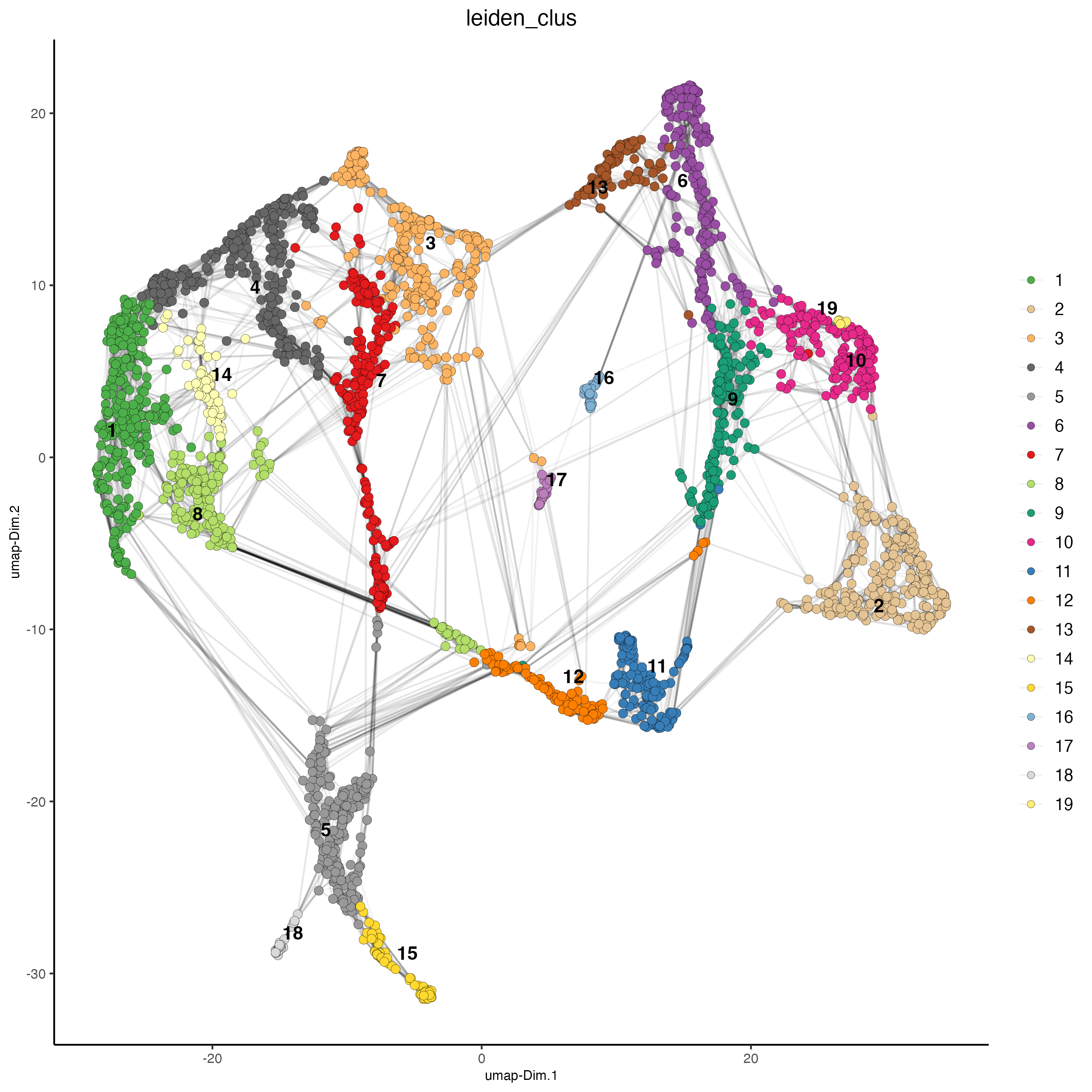
spatPlot2D(visium_brain,
           cell_color = "leiden_clus",
           coord_fix_ratio = 1)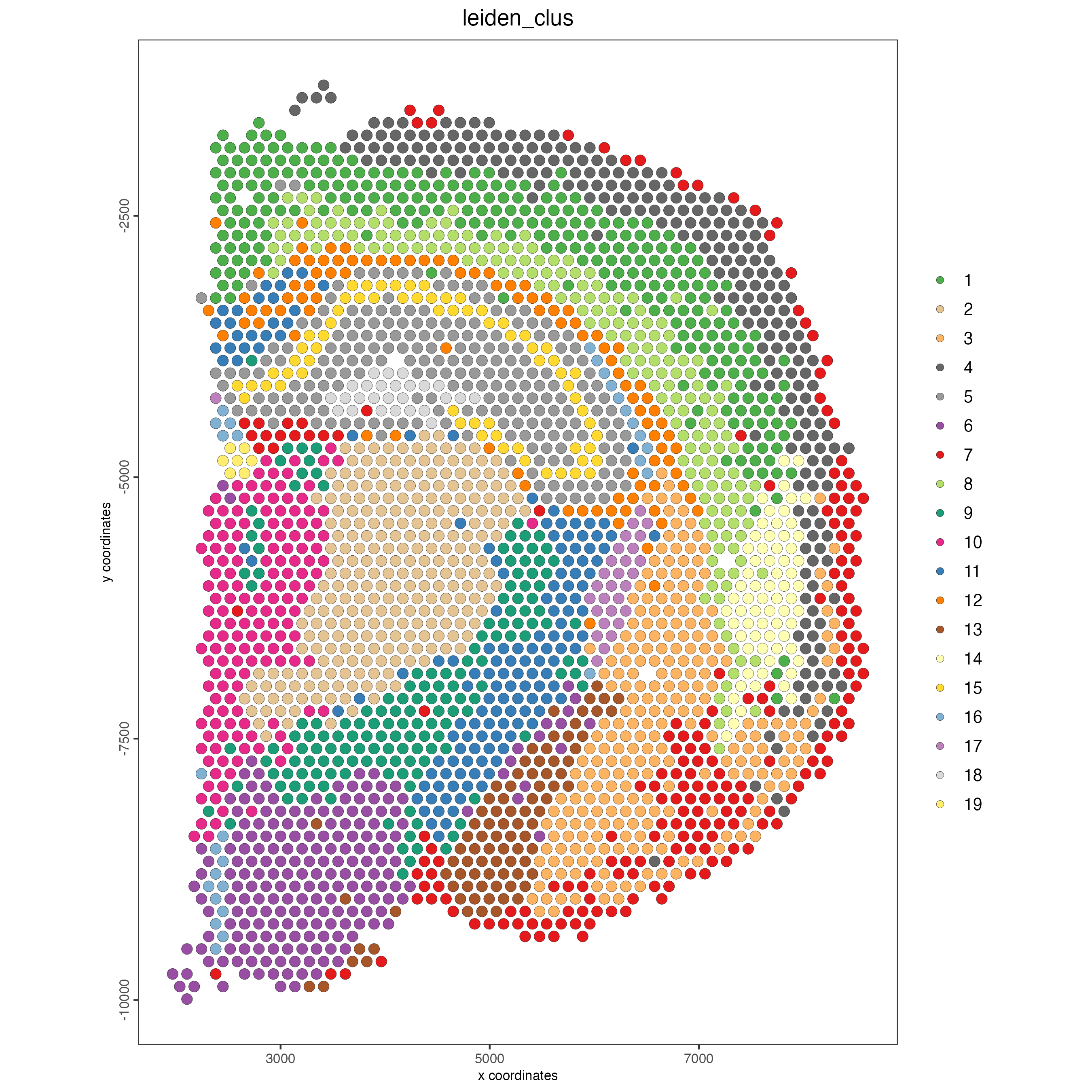
You can highlight one or more groups of interest:
spatPlot2D(visium_brain,
           cell_color = "leiden_clus",
           select_cell_groups = "8",
           coord_fix_ratio = 1,
           show_other_cells = TRUE,
           cell_color_code = c("8" = "red"),
           other_cell_color = "grey",
           other_point_size = 1.5)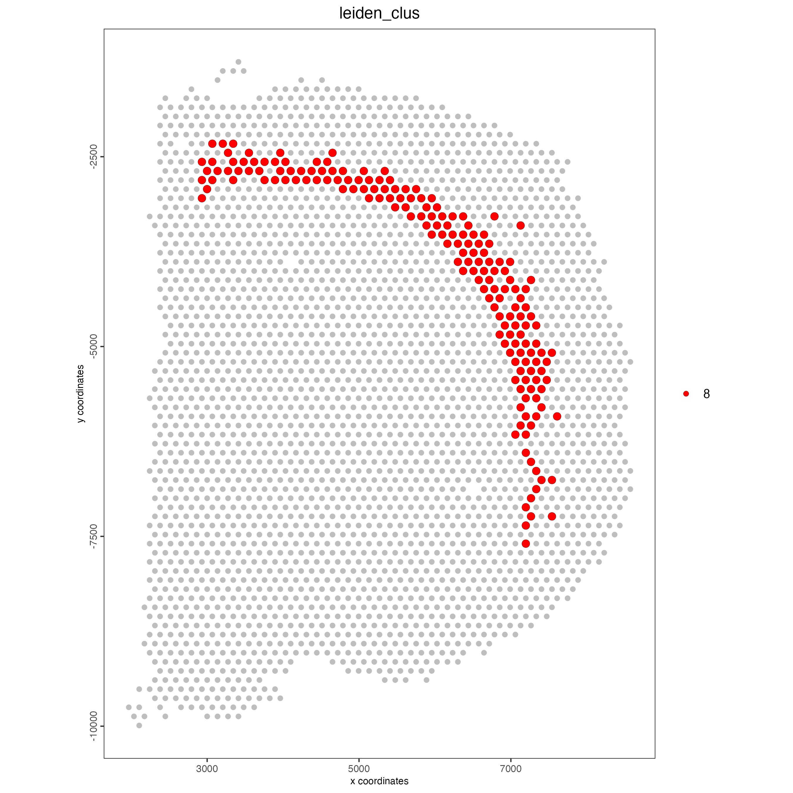
13 Subset data
If you want to take a deeper look at certain regions of the sample, use subsetGiottoLocs() and specify the axis ranges to create a sample subset.
# create and show subset
DG_subset <- subsetGiottoLocs(visium_brain,
                             x_max = 6500, x_min = 3000,
                             y_max = -2500, y_min = -5500,
                             return_gobject = TRUE)

spatDimPlot(gobject = DG_subset,
            cell_color = "leiden_clus",
            spat_point_size = 5)
14 Differential expression
14.1 Gini markers
The Gini method identifies genes that are very selectively expressed in a specific cluster, however not always expressed in all cells of that cluster. In other words, highly specific but not necessarily sensitive at the single-cell level.
- Calculate the top marker genes per cluster using the gini method.
gini_markers <- findMarkers_one_vs_all(gobject = visium_brain,
                                       method = "gini",
                                       expression_values = "normalized",
                                       cluster_column = "leiden_clus",
                                       min_feats = 10)

topgenes_gini <- gini_markers[, head(.SD, 2), by = "cluster"]$feats- Plot the normalized expression distribution of the top expressed genes.
violinPlot(visium_brain,
           feats = unique(topgenes_gini),
           cluster_column = "leiden_clus",
           strip_text = 6,
           strip_position = "right",
           save_param = list(base_width = 10, base_height = 30))
- Use the cluster IDs to create a heatmap with the normalized expression of the top expressed genes per cluster.
plotMetaDataHeatmap(visium_brain,
                    selected_feats = unique(topgenes_gini),
                    metadata_cols = "leiden_clus",
                    x_text_size = 10, y_text_size = 10)
- Visualize the scaled expression spatial distribution of the top expressed genes across the sample.
dimFeatPlot2D(visium_brain,
              expression_values = "scaled",
              feats = sort(unique(topgenes_gini)),
              cow_n_col = 5,
              point_size = 1,
              save_param = list(base_width = 15, base_height = 20))
14.2 Scran markers
The Scran method is preferred for robust differential expression analysis, especially when addressing technical variability or differences in sequencing depth across spatial locations.
- Calculate the top marker genes per cluster using the scran method.
scran_markers <- findMarkers_one_vs_all(gobject = visium_brain,
                                        method = "scran",
                                        expression_values = "normalized",
                                        cluster_column = "leiden_clus",
                                        min_feats = 10)

topgenes_scran <- scran_markers[, head(.SD, 2), by = "cluster"]$feats- Plot the normalized expression distribution of the top expressed genes.
violinPlot(visium_brain,
           feats = unique(topgenes_scran),
           cluster_column = "leiden_clus",
           strip_text = 6,
           strip_position = "right",
           save_param = list(base_width = 10, base_height = 30))
- Use the cluster IDs to create a heatmap with the normalized expression of the top expressed genes per cluster.
plotMetaDataHeatmap(visium_brain,
                    selected_feats = unique(topgenes_scran),
                    metadata_cols = "leiden_clus",
                    x_text_size = 10, y_text_size = 10)
- Visualize the scaled expression spatial distribution of the top expressed genes across the sample.
dimFeatPlot2D(visium_brain,
              expression_values = "scaled",
              feats = sort(unique(topgenes_scran)),
              cow_n_col = 5,
              point_size = 1,
              save_param = list(base_width = 20, base_height = 20))
In practice, it is often beneficial to apply both Gini and Scran methods and compare results for a more complete understanding of differential gene expression across clusters.
15 Cell type enrichment
Visium spatial transcriptomics does not provide single-cell resolution, making cell type annotation a harder problem. Giotto provides several ways to calculate enrichment of specific cell-type signature gene lists:
- PAGE
- hypergeometric test
- Rank
- DWLS Deconvolution Corresponded Single cell dataset can be generated from here.
The Giotto_SC object was processed from the downsampled Loom file and can also be downloaded from GiottoData::getSpatialDataset().
15.1 Download the single-cell dataset
GiottoData::getSpatialDataset(dataset = "scRNA_mouse_brain",
                              directory = data_path)
15.2 Create the single-cell object and run the normalization step
instructions <- createGiottoInstructions(
    save_dir = results_folder,
    save_plot = TRUE,
    show_plot = FALSE,
    python_path = python_path
)

sc_expression <- file.path(data_path, "brain_sc_expression_matrix.txt.gz")
sc_metadata <- file.path(data_path, "brain_sc_metadata.csv")

giotto_SC <- createGiottoObject(expression = sc_expression,
                                instructions = instructions)

cell_metadata <- data.table::fread(sc_metadata)

giotto_SC <- addCellMetadata(giotto_SC,
                             new_metadata = cell_metadata[, c("Class", "Subclass")])

giotto_SC <- normalizeGiotto(giotto_SC)
15.3 PAGE/Rank enrichment
Both Parametric Analysis of Gene Set Enrichment (PAGE) and Rank enrichment methods aim to determine whether a predefined set of genes show statistically significant differences in expression compared to other genes in the dataset.
15.3.1 Create PAGE matrix
The PAGE matrix should be a binary matrix where each row represents a gene marker and each column represents a cell type. There are several ways to create the PAGE matrix:
- Create binary matrix of cell signature genes
gran_markers <- c("Nr3c2", "Gabra5", "Tubgcp2", "Ahcyl2",
                  "Islr2", "Rasl10a", "Tmem114", "Bhlhe22",
                  "Ntf3", "C1ql2")

oligo_markers <- c("Efhd1", "H2-Ab1", "Enpp6", "Ninj2",
                   "Bmp4", "Tnr", "Hapln2", "Neu4",
                   "Wfdc18", "Ccp110")

di_mesench_markers <- c("Cartpt", "Scn1a", "Lypd6b",  "Drd5",
                        "Gpr88", "Plcxd2", "Cpne7", "Pou4f1",
                        "Ctxn2", "Wnt4")

sign_matrix <- makeSignMatrixPAGE(sign_names = c("Granule_neurons",
                                                 "Oligo_dendrocytes",
                                                 "di_mesenchephalon"),
                                  sign_list = list(gran_markers,
                                                   oligo_markers,
di_mesench_markers))- [shortcut] fully pre-prepared matrix for all cell types
sign_matrix_path <- system.file("extdata", "sig_matrix.txt",
                                package = "GiottoData")

brain_sc_markers <- data.table::fread(sign_matrix_path)

sign_matrix <- as.matrix(brain_sc_markers[,-1])
rownames(sign_matrix) <- brain_sc_markers$Event- make a PAGE matrix from single cell dataset
markers_scran <- findMarkers_one_vs_all(gobject = giotto_SC,
                                        method = "scran",
                                        expression_values = "normalized",
                                        cluster_column = "Class",
                                        min_feats = 3)

top_markers <- markers_scran[, head(.SD, 10), by = "cluster"]
celltypes <- levels(factor(markers_scran$cluster))

sign_list <- list()

for (i in 1:length(celltypes)){
  sign_list[[i]] = top_markers[which(top_markers$cluster == celltypes[i]),]$feats
}

sign_matrix <- makeSignMatrixPAGE(sign_names = celltypes,
                                  sign_list = sign_list)
15.3.2 Run the enrichment test with PAGE
runSpatialEnrich() can also be used as a wrapper for all currently provided enrichment options.
visium_brain <- runPAGEEnrich(gobject = visium_brain,
sign_matrix = sign_matrix)- Create a heatmap showing the enrichment of cell types (from the single-cell data annotation) in the spatial dataset clusters.
cell_types_PAGE <- colnames(sign_matrix)

plotMetaDataCellsHeatmap(gobject = visium_brain,
                         metadata_cols = "leiden_clus",
                         value_cols = cell_types_PAGE,
                         spat_enr_names = "PAGE",
                         x_text_size = 8,
                         y_text_size = 8)
- Plot the spatial distribution of the cell types.
spatCellPlot2D(gobject = visium_brain,
               spat_enr_names = "PAGE",
               cell_annotation_values = cell_types_PAGE,
               cow_n_col = 3,
               coord_fix_ratio = 1,
               point_size = 1,
               show_legend = TRUE)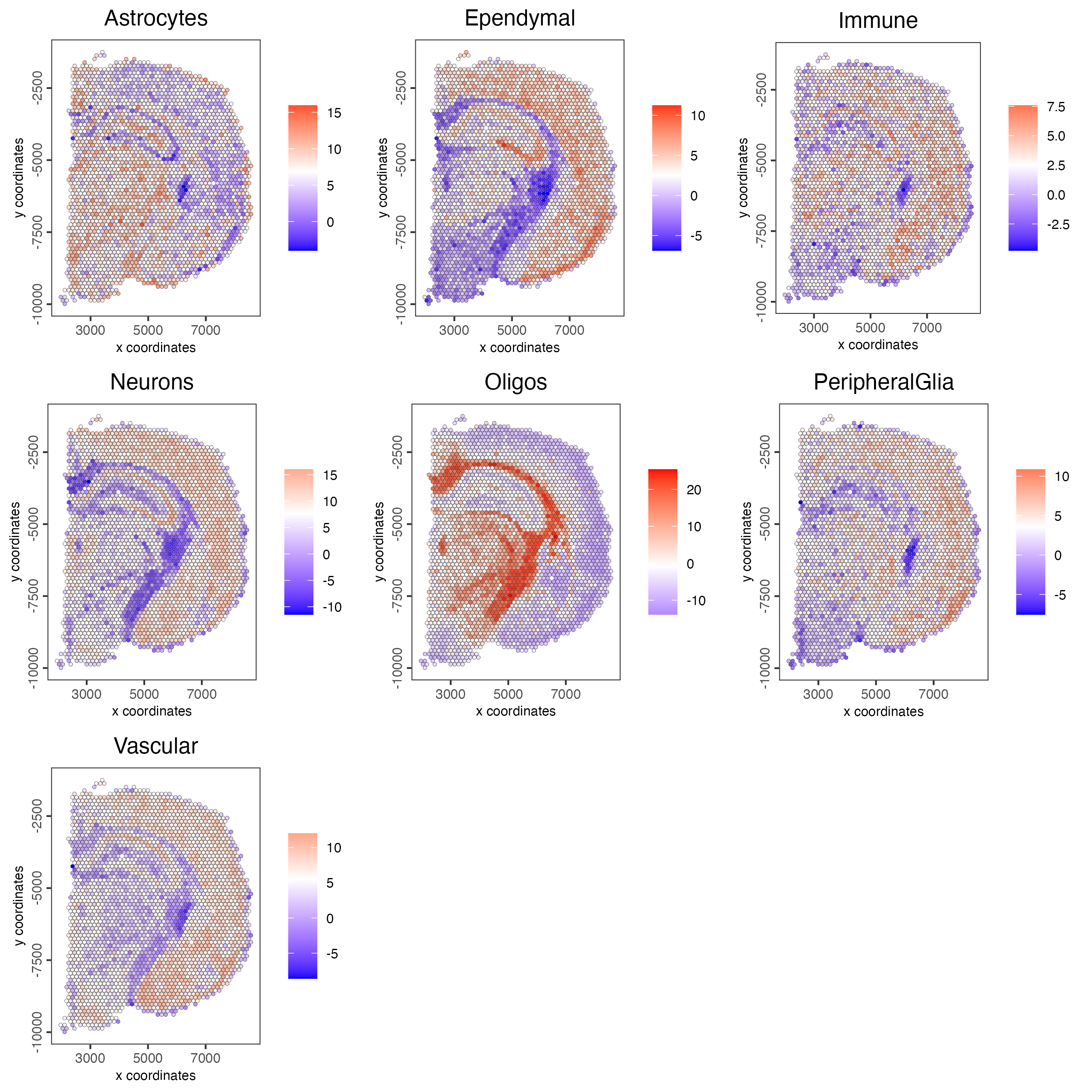
15.4 HyperGeometric test
The hypergeometric test has been widely used for searching gene overrepresentation in categories such as diseases or particular Gene Ontology (GO) terms for cellular compartments, molecular functions, or biological processes. Traditionally, enrichment analysis with the hypergeometric test asks the question “What is the probability that k or more out of n genes associated with the pathway are in a list of length N, where those N genes are sampled from a background of size M?” You can find more information about this test here
visium_brain <- runHyperGeometricEnrich(gobject = visium_brain,
                                        expression_values = "normalized",
                                        sign_matrix = sign_matrix)

cell_types_HyperGeometric <- colnames(sign_matrix)

spatCellPlot(gobject = visium_brain,
             spat_enr_names = "hypergeometric",
             cell_annotation_values = cell_types_HyperGeometric[1:4],
             cow_n_col = 2,
             coord_fix_ratio = NULL,
             point_size = 1.75)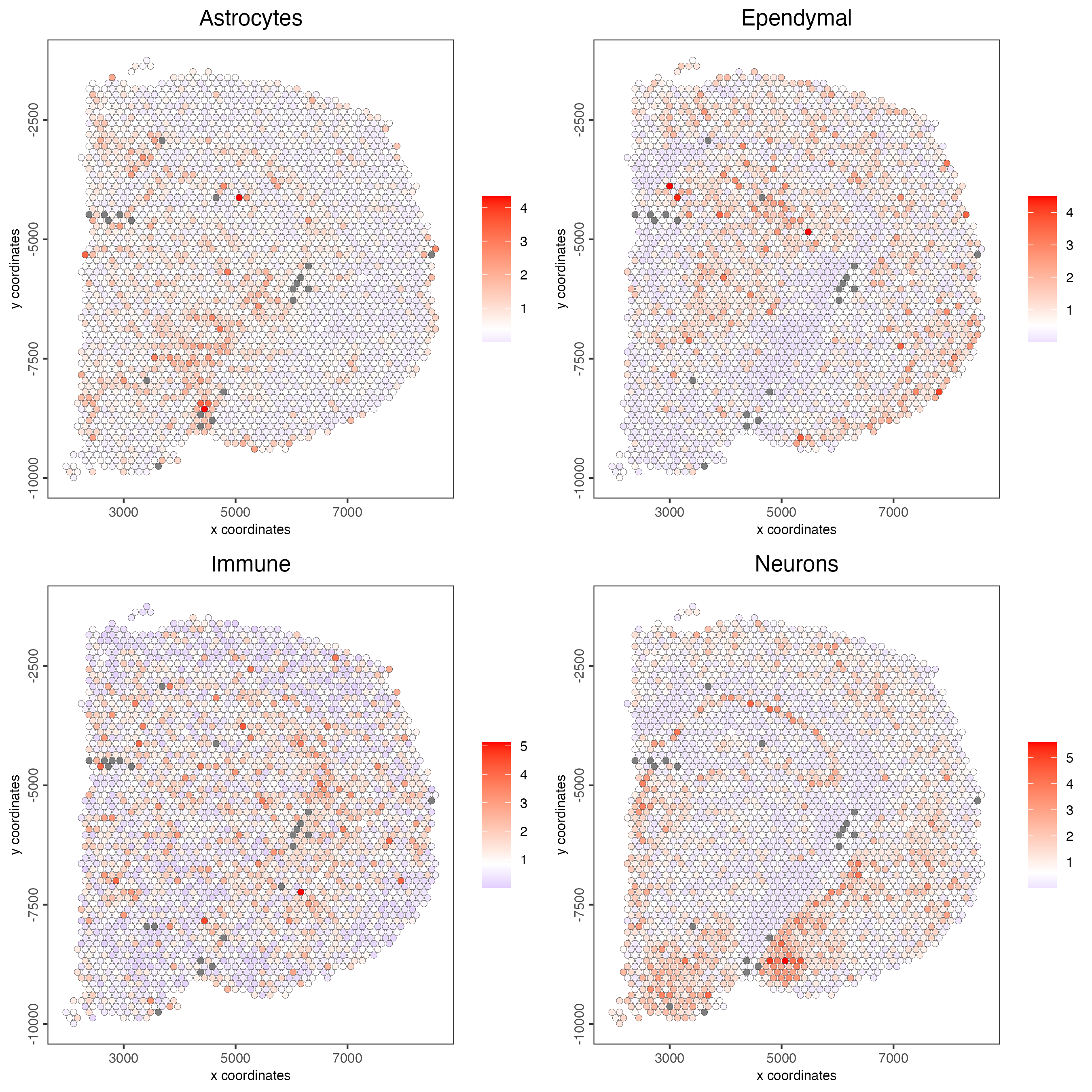
15.5 Rank enrichment
In this method, enrichment is calculated based on the rank of fold-change for each gene in each spot and the rank of each marker in each cell type.
15.5.1 Create rank matrix
Note that rank matrix is different from PAGE. A count matrix and a vector for all cell labels will be needed.
rank_matrix <- makeSignMatrixRank(sc_matrix = getExpression(giotto_SC,
                                                            values = "normalized",
                                                            output = "matrix"),
                                  sc_cluster_ids = pDataDT(giotto_SC)$Class)

colnames(rank_matrix) <- levels(factor(pDataDT(giotto_SC)$Class))
15.5.2 Run Rank enrichment
visium_brain <- runRankEnrich(gobject = visium_brain,
                              sign_matrix = rank_matrix,
                              expression_values = "normalized")

# Plot Rank enrichment result
spatCellPlot2D(gobject = visium_brain,
               spat_enr_names = "rank",
               cell_annotation_values = colnames(rank_matrix)[1:4],
               cow_n_col = 2,
               coord_fix_ratio = 1,
               point_size = 1)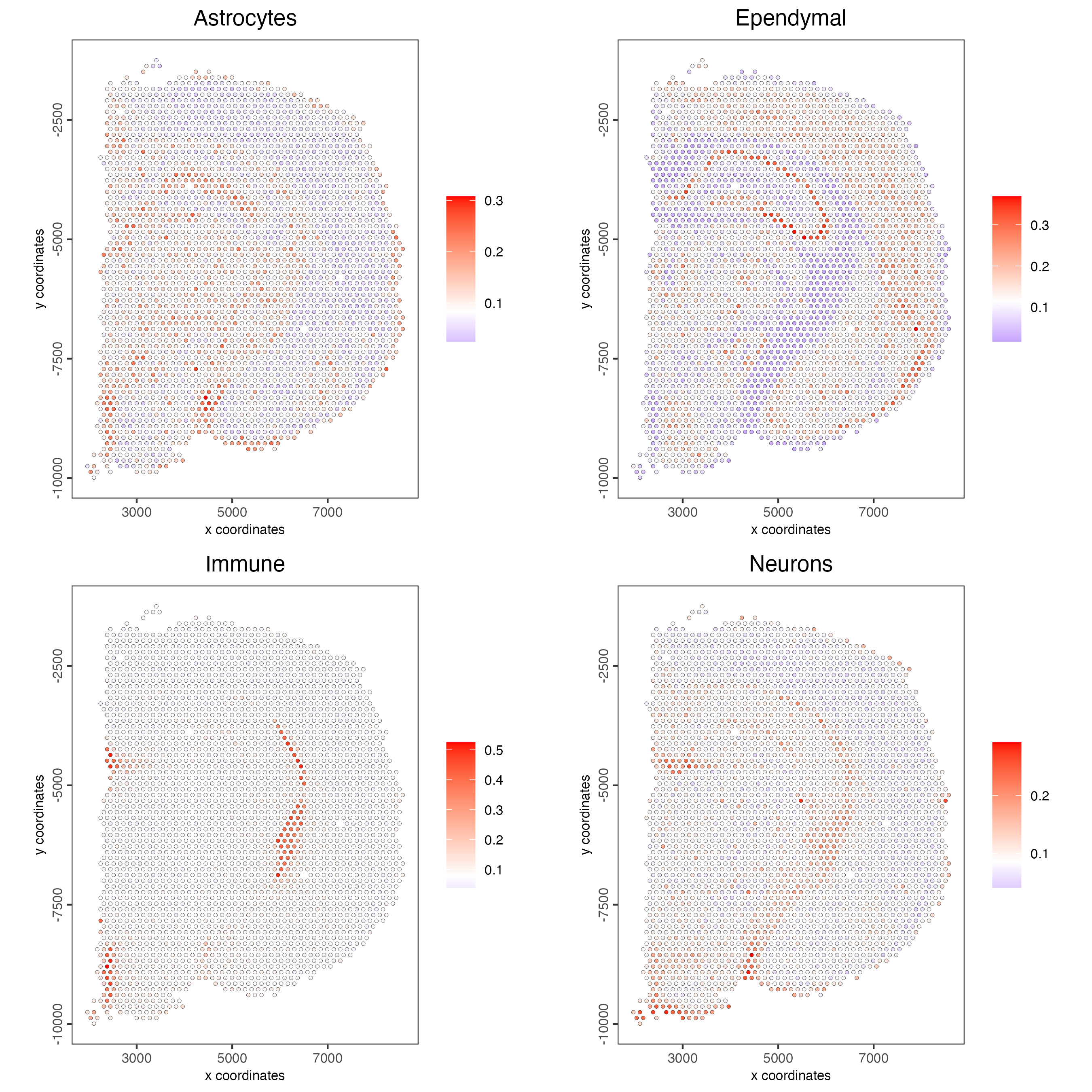
15.6 DWLS spatial deconvolution
Spatial Dampened Weighted Least Squares (DWLS) estimates the proportions of different cell types across spots in a tissue.
15.6.1 Create DWLS matrix
Note that DWLS matrix is different from PAGE and rank. A count matrix a vector for a list of gene signatures and a vector for all cell labels will be needed.
DWLS_matrix <- makeSignMatrixDWLSfromMatrix(
  matrix = getExpression(giotto_SC,
                         values = "normalized",
                         output = "matrix"),
  cell_type = pDataDT(giotto_SC)$Class,
  sign_gene = topgenes_scran)
15.6.2 Run DWLS deconvolution
visium_brain <- runDWLSDeconv(gobject = visium_brain,
sign_matrix = DWLS_matrix)- Plot the DWLS deconvolution result coloring by the proportion of a certain cell type per spot.
spatCellPlot2D(gobject = visium_brain,
               spat_enr_names = "DWLS",
               cell_annotation_values = levels(factor(pDataDT(giotto_SC)$Class))[1:4],
               cow_n_col = 2,
               coord_fix_ratio = 1,
               point_size = 1)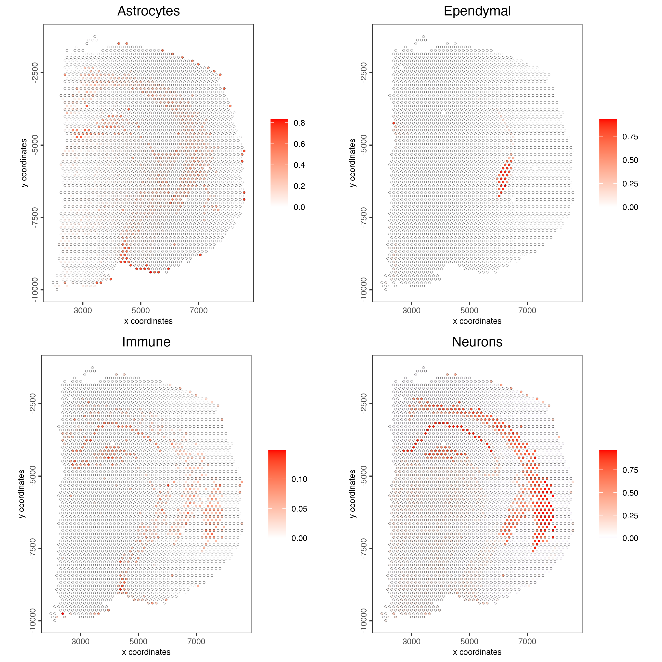
- Plot the DWLS deconvolution result creating with pie plots showing the proportion of each cell type per spot.
spatDeconvPlot(visium_brain,
               show_image = TRUE,
               radius = 50)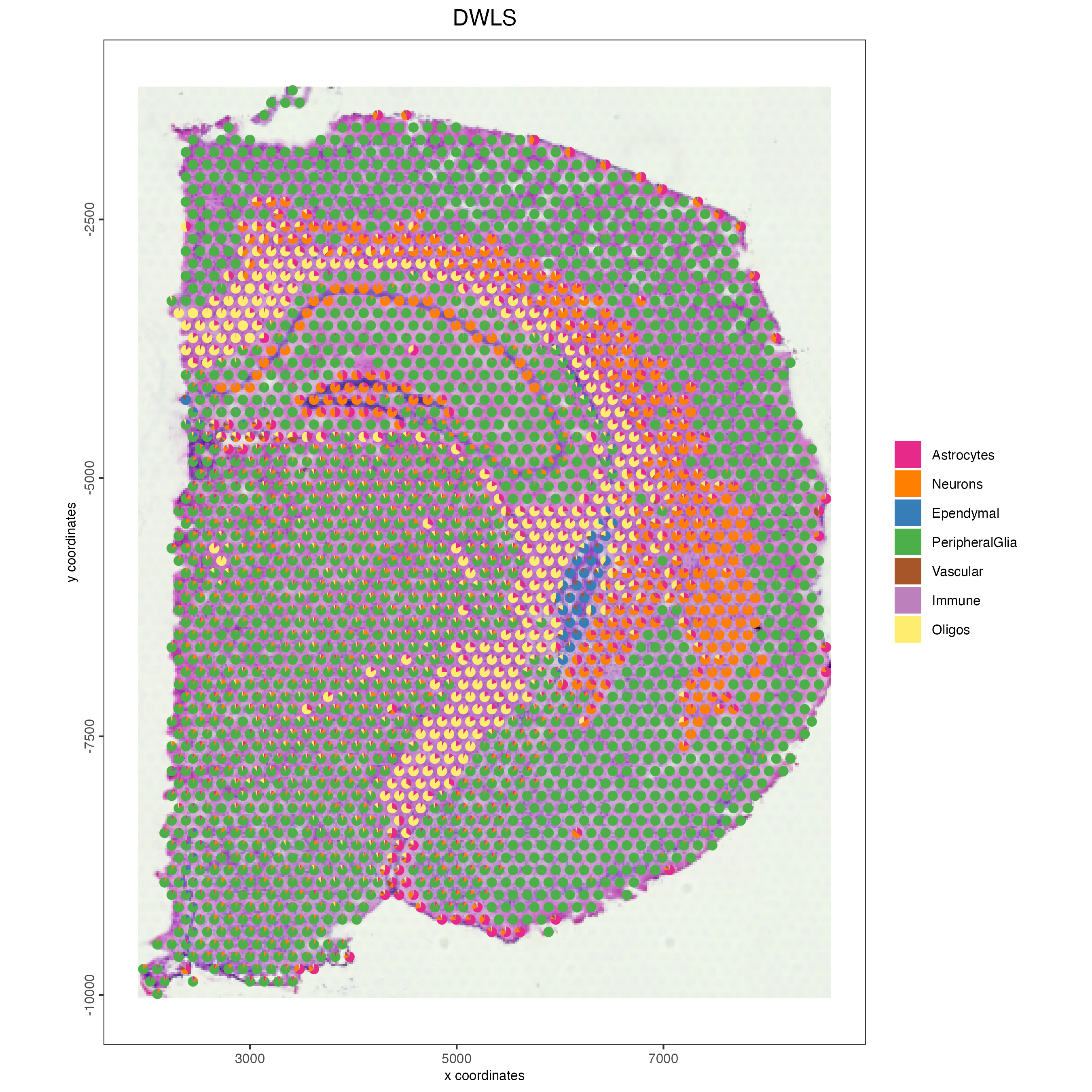
16 Spatial grid
Create spatial grids by specifying the step size in both axis. This information will be saved in the Giotto object.
visium_brain <- createSpatialGrid(gobject = visium_brain,
                                  sdimx_stepsize = 400,
                                  sdimy_stepsize = 400,
                                  minimum_padding = 0)

showGiottoSpatGrids(visium_brain)

spatPlot2D(visium_brain,
           cell_color = "leiden_clus",
           show_grid = TRUE,
           grid_color = "red",
           spatial_grid_name = "spatial_grid")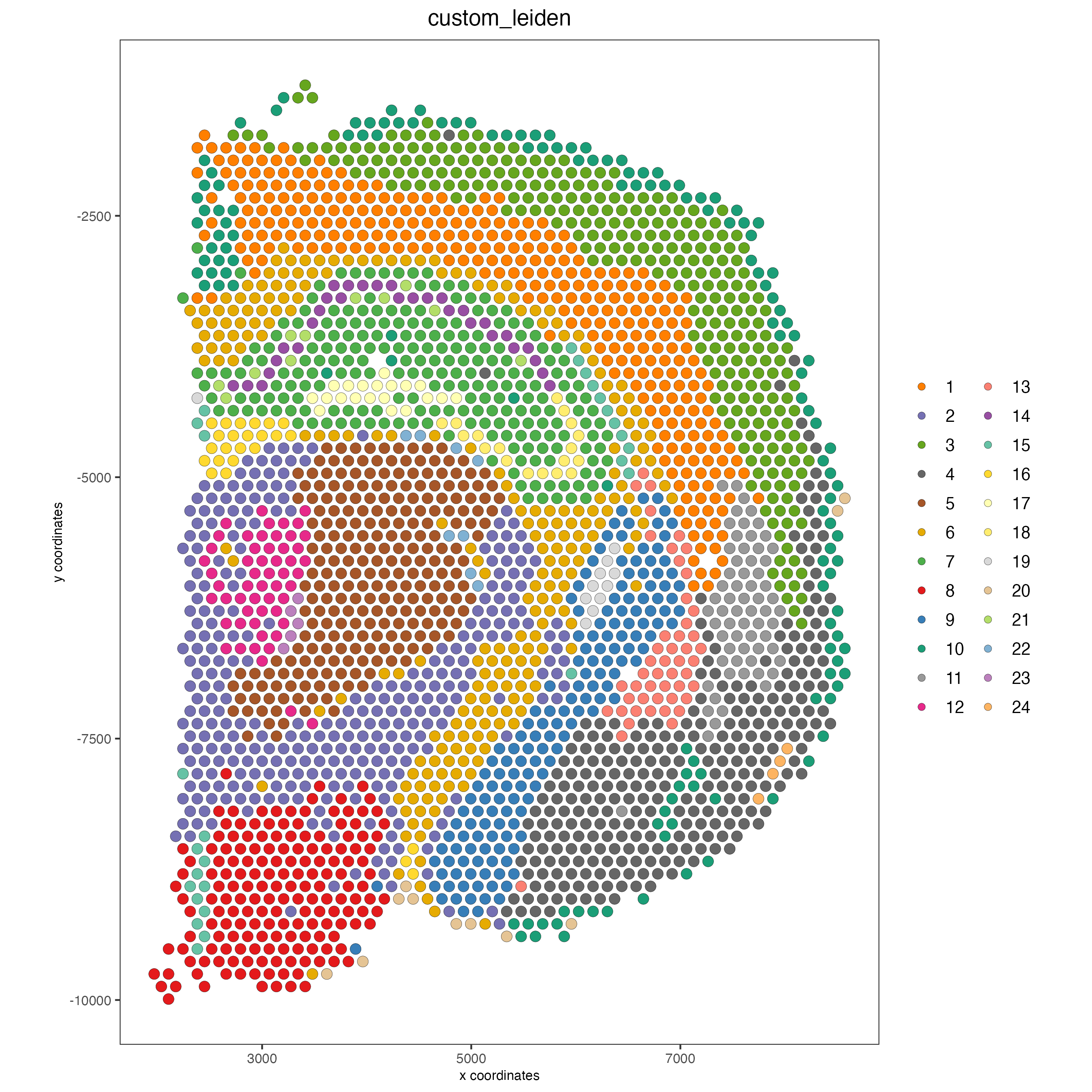
17 Spatial expression patterns
When having the spatial location of each spot/cell, you can look for genes that follow and share particular spatial distributions.
17.1 Create a spatial network
createSpatialNetwork() creates a spatial network connecting single-cells based on their physical distance to each other. There are two methods available: Delaunay and kNN. For the Delaunay method, neighbors will be decided by Delaunay triangulation and a maximum distance criterion. For the kNN method, the number of neighbors can be determined by k, or the maximum distance from each cell with or without setting a minimum k for each cell.
visium_brain <- createSpatialNetwork(gobject = visium_brain,
                                     method = "kNN",
                                     k = 6,
                                     maximum_distance_knn = 400,
                                     name = "spatial_network")

spatPlot2D(gobject = visium_brain,
           show_network= TRUE,
           network_color = "blue",
           spatial_network_name = "spatial_network")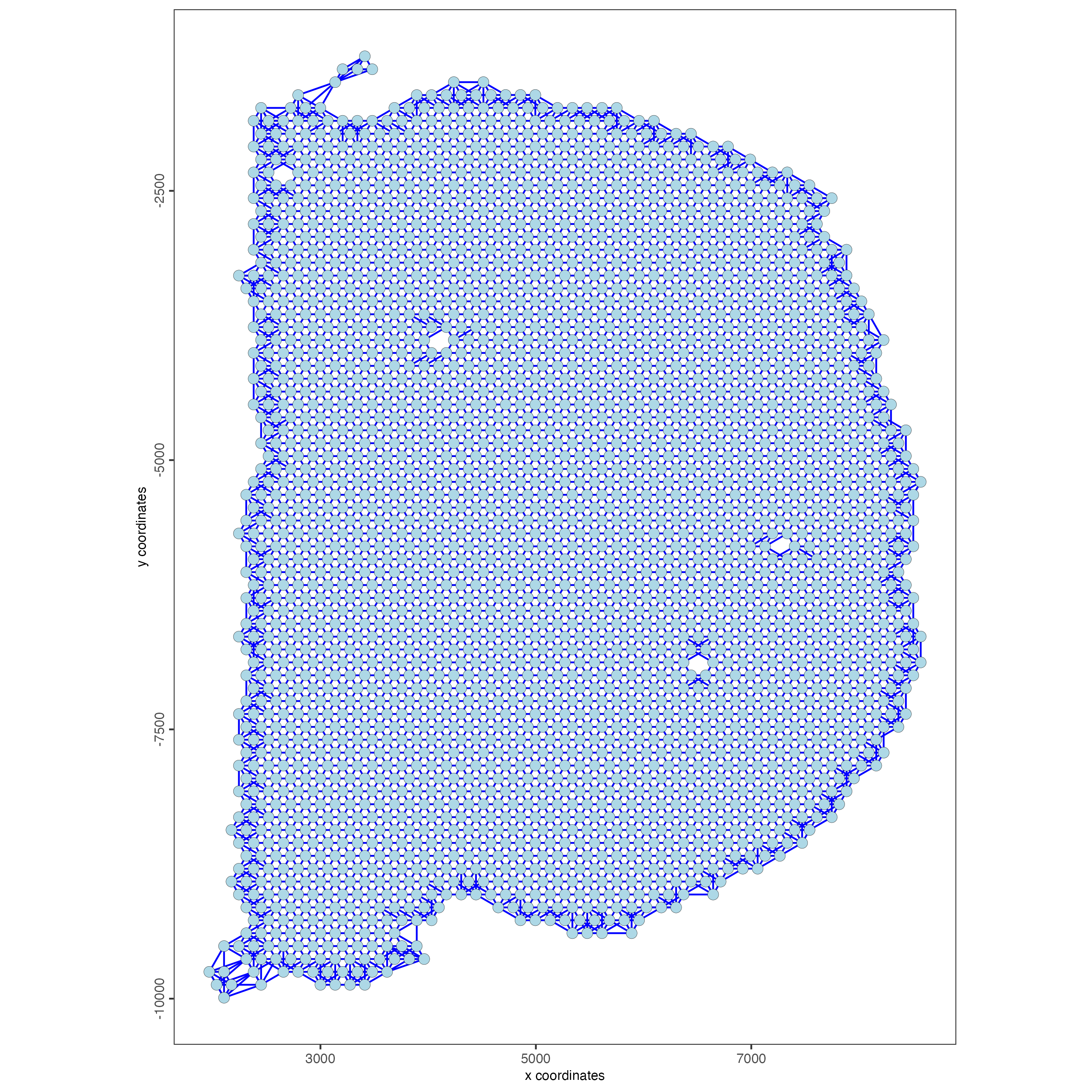
17.2 Find spatial genes
Use the rank binarization to rank genes on the spatial dataset depending on whether they exhibit a spatial pattern location or not. This step may take a few minutes to run.
ranktest <- binSpect(visium_brain,
                     bin_method = "rank",
                     calc_hub = TRUE,
                     hub_min_int = 5,
spatial_network_name = "spatial_network")- Plot the scaled expression of genes with the highest probability of being spatial genes.
spatFeatPlot2D(visium_brain,
               expression_values = "scaled",
               feats = ranktest$feats[1:6],
               cow_n_col = 2,
               point_size = 1)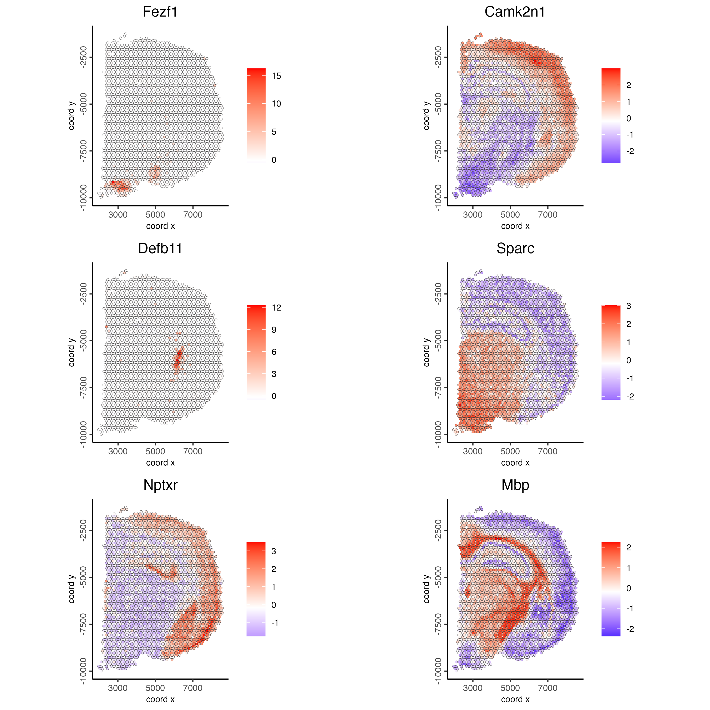
17.3 Spatial Co-Expression modules
Once we have found spatial genes, we can group those genes with similar spatial patterns into co-expression modules.
- Cluster the top 500 spatial genes into 20 clusters
ext_spatial_genes <- ranktest[1:500,]$feats- Use detectSpatialCorGenes() to calculate pairwise distances between genes.
spat_cor_netw_DT <- detectSpatialCorFeats(
    visium_brain,
    method = "network",
    spatial_network_name = "spatial_network",
subset_feats = ext_spatial_genes)- Identify most similar spatially correlated genes for one gene.
top10_genes <- showSpatialCorFeats(spat_cor_netw_DT,
                                  feats = "Mbp",
show_top_feats = 10)- Plot the scaled expression of the 3 genes with most similar spatial patterns to Mbp.
spatFeatPlot2D(visium_brain,
               expression_values = "scaled",
               feats = top10_genes$variable[1:4],
               point_size = 1.5)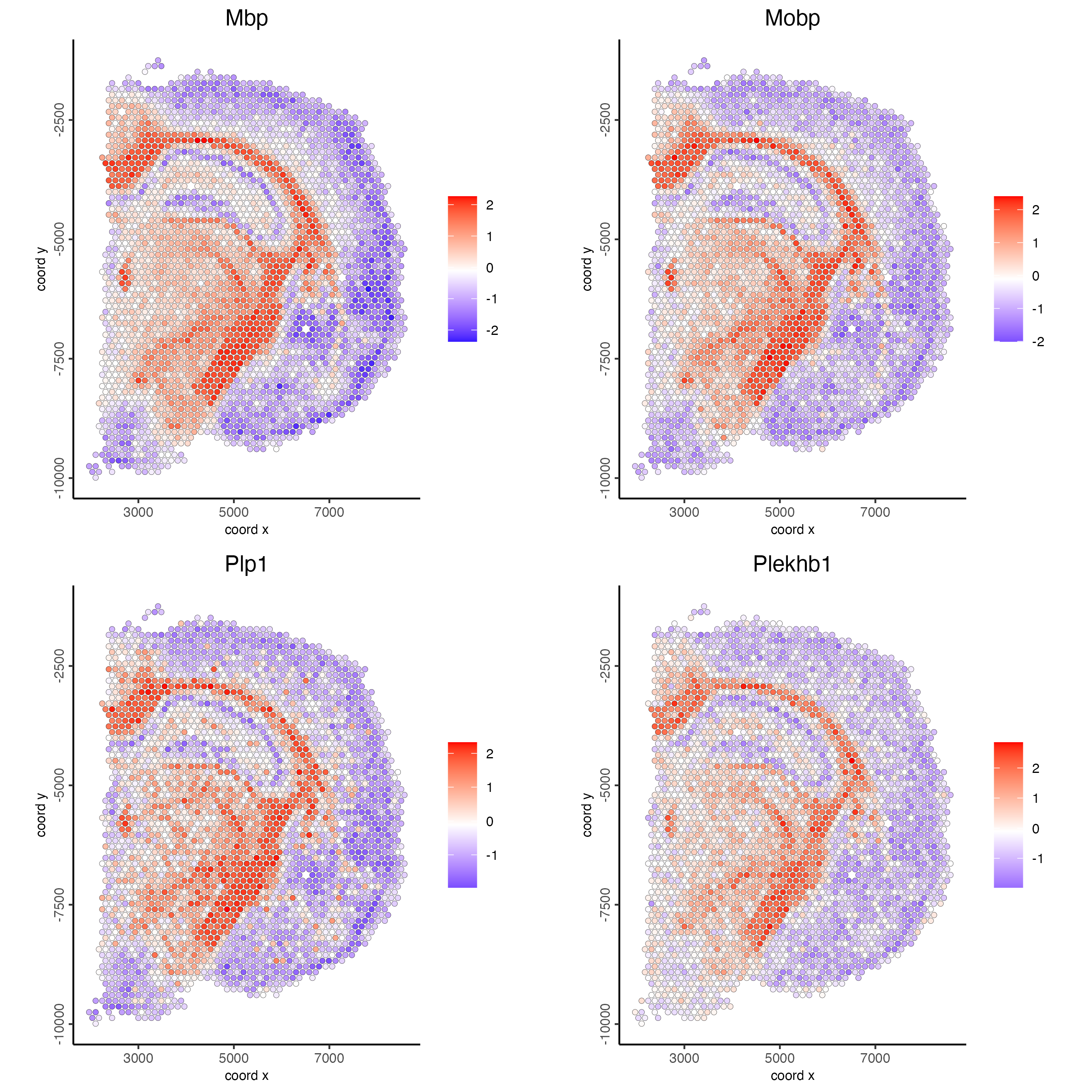
- Cluster spatial genes.
spat_cor_netw_DT <- clusterSpatialCorFeats(spat_cor_netw_DT,
                                           name = "spat_netw_clus",
k = 20)- Plot the correlation of the top 500 spatial genes with their assigned cluster.
heatmSpatialCorFeats(visium_brain,
                     spatCorObject = spat_cor_netw_DT,
                     use_clus_name = "spat_netw_clus",
                     heatmap_legend_param = list(title = NULL))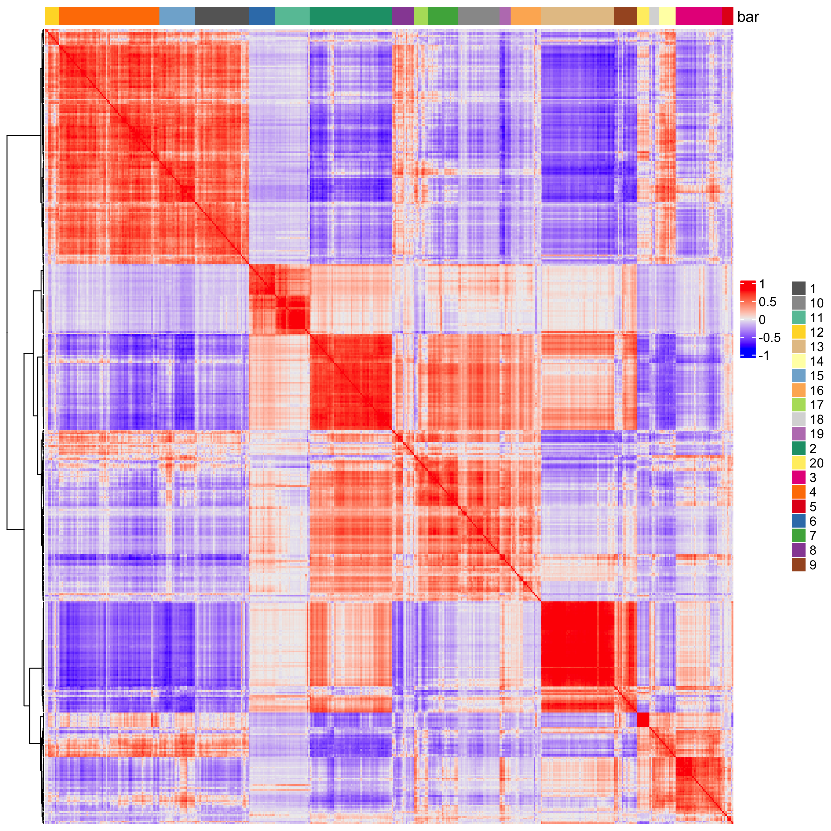
- Rank spatial correlated clusters and show genes for selected clusters.
netw_ranks <- rankSpatialCorGroups(
  visium_brain,
  spatCorObject = spat_cor_netw_DT,
use_clus_name = "spat_netw_clus")- Plot the correlation and number of spatial genes in each cluster.
top_netw_spat_cluster <- showSpatialCorFeats(spat_cor_netw_DT,
                                            use_clus_name = "spat_netw_clus",
                                            selected_clusters = 6,
                                            show_top_feats = 1)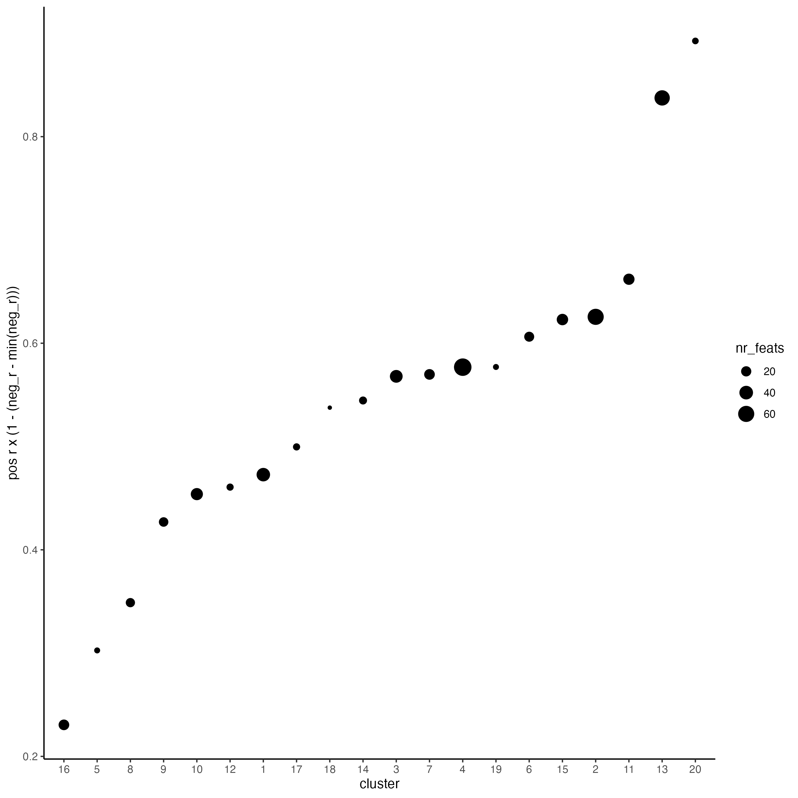
- Create the metagene enrichment score per co-expression cluster.
cluster_genes_DT <- showSpatialCorFeats(spat_cor_netw_DT,
                                        use_clus_name = "spat_netw_clus",
                                        show_top_feats = 1)

cluster_genes <- cluster_genes_DT$clus
names(cluster_genes) <- cluster_genes_DT$feat_ID

visium_brain <- createMetafeats(visium_brain,
                                feat_clusters = cluster_genes,
name = "cluster_metagene")- Plot the spatial distribution of the metagene enrichment scores of each spatial co-expression cluster.
spatCellPlot(visium_brain,
             spat_enr_names = "cluster_metagene",
             cell_annotation_values = netw_ranks$clusters,
             point_size = 1,
             cow_n_col = 5)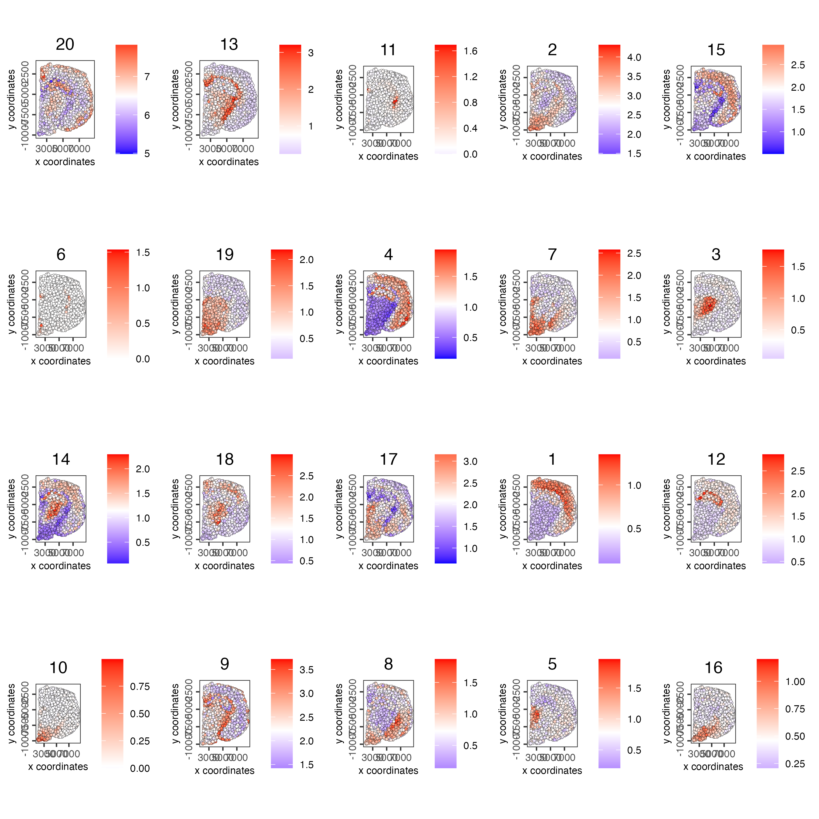
18 Spatially informed clusters
Once we identified spatial genes, we can use them to re-calculate the clusters based only on the expression information that follows spatial patterns.
18.1 Get the top 30 genes per spatial co-expression cluster
coexpr_dt <- data.table::data.table(
  genes = names(spat_cor_netw_DT$cor_clusters$spat_netw_clus),
  cluster = spat_cor_netw_DT$cor_clusters$spat_netw_clus)

data.table::setorder(coexpr_dt, cluster)

top30_coexpr_dt <- coexpr_dt[, head(.SD, 30) , by = cluster]

spatial_genes <- top30_coexpr_dt$genes
18.2 Re-calculate the clustering
Use the spatial genes to calculate again the principal components, umap, network and clustering.
visium_brain <- runPCA(gobject = visium_brain,
                       feats_to_use = spatial_genes,
                       name = "custom_pca")

visium_brain <- runUMAP(visium_brain,
                        dim_reduction_name = "custom_pca",
                        dimensions_to_use = 1:20,
                        name = "custom_umap")

visium_brain <- createNearestNetwork(gobject = visium_brain,
                                     dim_reduction_name = "custom_pca",
                                     dimensions_to_use = 1:20,
                                     k = 5,
                                     name = "custom_NN")

visium_brain <- doLeidenCluster(gobject = visium_brain,
                                network_name = "custom_NN",
                                resolution = 0.15,
                                n_iterations = 1000,
name = "custom_leiden")- Plot the spatial distribution of the Leiden clusters calculated based on the spatial genes.
spatPlot2D(visium_brain,
           cell_color = "custom_leiden",
           point_size = 3)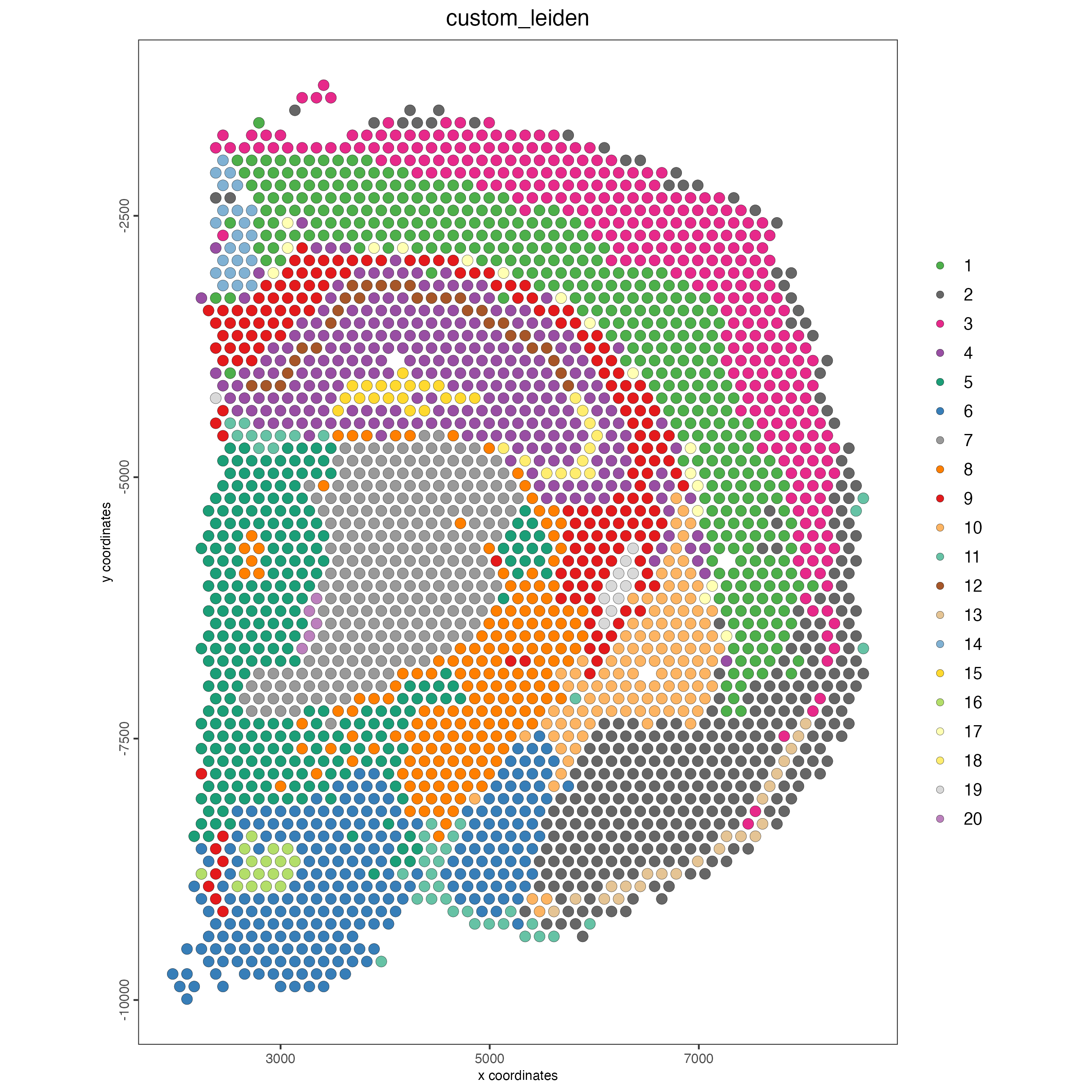
- Plot the UMAP and color the spots using the Leiden clusters calculated based on the spatial genes.
plotUMAP(gobject = visium_brain,
         cell_color = "custom_leiden")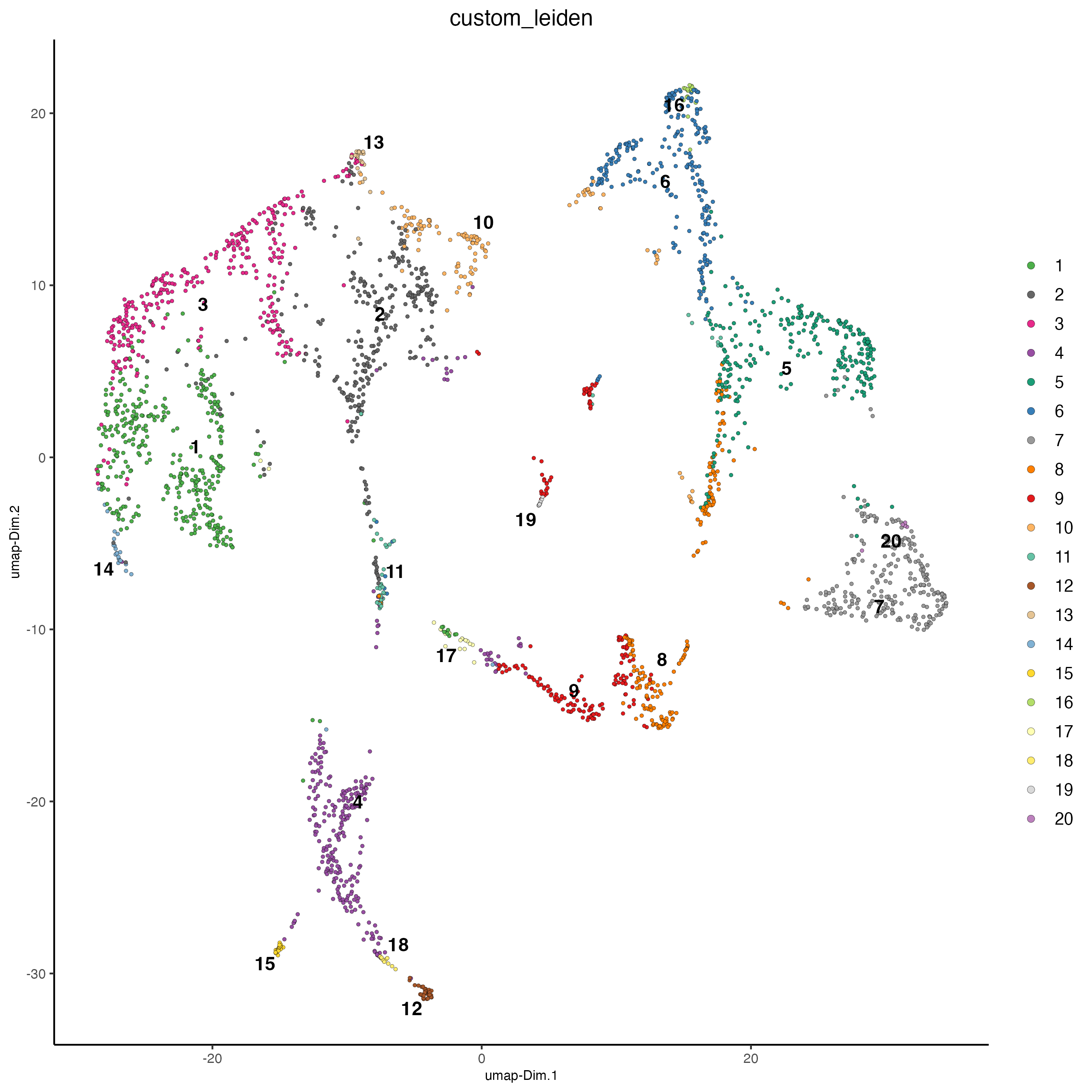
19 Spatial domains with HMRF
Hidden Markov Random Field (HMRF) models capture spatial dependencies and segment tissue regions based on shared and gene expression patterns.
- Run HMRF with different betas on top 30 genes per spatial co-expression module. This step may take several minutes to run.
hmrf_folder <- file.path(results_folder, "HMRF")

if(!file.exists(hmrf_folder)) dir.create(hmrf_folder, recursive = TRUE)

HMRF_spatial_genes <- doHMRF(gobject = visium_brain,
                            expression_values = "scaled",
                            spatial_genes = spatial_genes,
                            k = 20,
                            spatial_network_name="spatial_network",
                            betas = c(0, 10, 5),
output_folder = hmrf_folder)- Add the HMRF results to the giotto object
visium_brain <- addHMRF(gobject = visium_brain,
                        HMRFoutput = HMRF_spatial_genes,
                        k = 20,
                        betas_to_add = c(0, 10, 20, 30, 40),
hmrf_name = "HMRF")- Plot the spatial distribution of the HMRF domains.
spatPlot2D(gobject = visium_brain,
           cell_color = "HMRF_k20_b.40")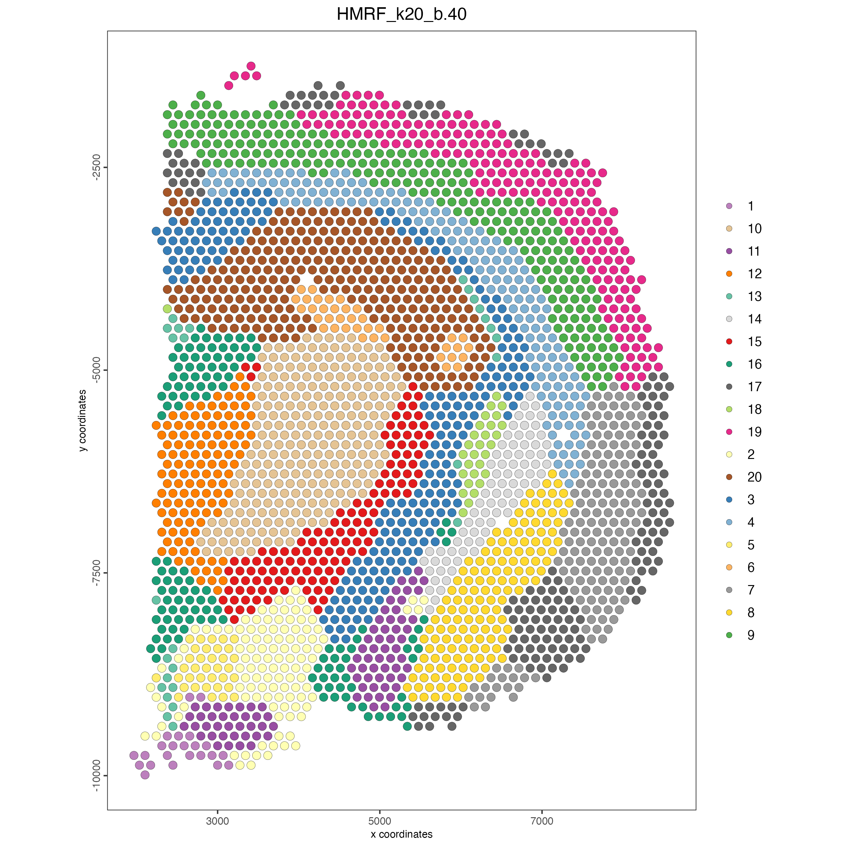
20 Session info
R version 4.4.2 (2024-10-31)
Platform: x86_64-apple-darwin20
Running under: macOS Sequoia 15.4

Matrix products: default
BLAS:   /System/Library/Frameworks/Accelerate.framework/Versions/A/Frameworks/vecLib.framework/Versions/A/libBLAS.dylib
LAPACK: /Library/Frameworks/R.framework/Versions/4.4-x86_64/Resources/lib/libRlapack.dylib;  LAPACK version 3.12.0

locale:
[1] en_US.UTF-8/en_US.UTF-8/en_US.UTF-8/C/en_US.UTF-8/en_US.UTF-8

time zone: America/New_York
tzcode source: internal

attached base packages:
[1] stats     graphics  grDevices utils     datasets  methods   base

other attached packages:
[1] Giotto_4.2.1      GiottoClass_0.4.7

loaded via a namespace (and not attached):
  [1] RColorBrewer_1.1-3          shape_1.4.6.1               rstudioapi_0.17.1
  [4] jsonlite_2.0.0              magrittr_2.0.3              magick_2.8.6
  [7] farver_2.1.2                rmarkdown_2.29              GlobalOptions_0.1.2
 [10] zlibbioc_1.52.0             ragg_1.3.3                  vctrs_0.6.5
 [13] Cairo_1.6-2                 memoise_2.0.1               GiottoUtils_0.2.4
 [16] terra_1.8-29                htmltools_0.5.8.1           S4Arrays_1.6.0
 [19] BiocNeighbors_2.0.1         SparseArray_1.6.2           parallelly_1.43.0
 [22] htmlwidgets_1.6.4           plotly_4.10.4               cachem_1.1.0
 [25] igraph_2.1.4                iterators_1.0.14            lifecycle_1.0.4
 [28] pkgconfig_2.0.3             rsvd_1.0.5                  Matrix_1.7-3
 [31] R6_2.6.1                    fastmap_1.2.0               clue_0.3-66
 [34] GenomeInfoDbData_1.2.13     MatrixGenerics_1.18.1       future_1.34.0
 [37] digest_0.6.37               colorspace_2.1-1            S4Vectors_0.44.0
 [40] dqrng_0.4.1                 irlba_2.3.5.1               textshaping_1.0.0
 [43] GenomicRanges_1.58.0        beachmat_2.22.0             labeling_0.4.3
 [46] progressr_0.15.1            httr_1.4.7                  polyclip_1.10-7
 [49] abind_1.4-8                 compiler_4.4.2              doParallel_1.0.17
 [52] withr_3.0.2                 backports_1.5.0             BiocParallel_1.40.0
 [55] viridis_0.6.5               ggforce_0.4.2               R.utils_2.13.0
 [58] MASS_7.3-65                 DelayedArray_0.32.0         rjson_0.2.23
 [61] bluster_1.16.0              gtools_3.9.5                GiottoVisuals_0.2.12
 [64] tools_4.4.2                 future.apply_1.11.3         quadprog_1.5-8
 [67] R.oo_1.27.0                 glue_1.8.0                  dbscan_1.2.2
 [70] grid_4.4.2                  checkmate_2.3.2             Rtsne_0.17
 [73] cluster_2.1.8.1             generics_0.1.3              gtable_0.3.6
 [76] R.methodsS3_1.8.2           tidyr_1.3.1                 data.table_1.17.0
 [79] BiocSingular_1.22.0         tidygraph_1.3.1             ScaledMatrix_1.14.0
 [82] metapod_1.14.0              XVector_0.46.0              BiocGenerics_0.52.0
 [85] foreach_1.5.2               ggrepel_0.9.6               pillar_1.10.1
 [88] limma_3.62.2                circlize_0.4.16             dplyr_1.1.4
 [91] tweenr_2.0.3                lattice_0.22-6              FNN_1.1.4.1
 [94] tidyselect_1.2.1            ComplexHeatmap_2.22.0       SingleCellExperiment_1.28.1
 [97] locfit_1.5-9.12             scuttle_1.16.0              knitr_1.50
[100] gridExtra_2.3               IRanges_2.40.1              edgeR_4.4.2
[103] SummarizedExperiment_1.36.0 scattermore_1.2             stats4_4.4.2
[106] xfun_0.51                   graphlayouts_1.2.2          Biobase_2.66.0
[109] statmod_1.5.0               matrixStats_1.5.0           UCSC.utils_1.2.0
[112] lazyeval_0.2.2              yaml_2.3.10                 evaluate_1.0.3
[115] codetools_0.2-20            ggraph_2.2.1                GiottoData_0.2.16
[118] tibble_3.2.1                colorRamp2_0.1.0            cli_3.6.4
[121] RcppParallel_5.1.10         uwot_0.2.3                  reticulate_1.42.0
[124] systemfonts_1.2.1           munsell_0.5.1               Rcpp_1.0.14
[127] GenomeInfoDb_1.42.3         zigg_0.0.2                  globals_0.16.3
[130] png_0.1-8                   Rfast_2.1.5.1               parallel_4.4.2
[133] ggplot2_3.5.1               scran_1.34.0                sparseMatrixStats_1.18.0
[136] listenv_0.9.1               SpatialExperiment_1.16.0    viridisLite_0.4.2
[139] scales_1.3.0                purrr_1.0.4                 crayon_1.5.3
[142] GetoptLong_1.0.5            rlang_1.1.5                 cowplot_1.1.3