Xenium Human Breast Cancer Pre-Release
Source:vignettes/xenium_breast_cancer.rmd
xenium_breast_cancer.rmdThis is a legacy dataset.
For a more recent example, see Xenium FFPE Human Lung Cancer with Multimodal Cell Segmentation
1 Install Extra Packages
1.1 arrow installation
Xenium datasets requires arrow with ZTSD support to be installed to work with parquet files. This is optional if you want to use a different format for the tabular data.
has_arrow <- requireNamespace("arrow", quietly = TRUE)
zstd <- TRUE
if (has_arrow) {
    # check arrow_info() to see that zstd support should be TRUE
    # See https://arrow.apache.org/docs/r/articles/install.html for details
    zstd <- arrow::arrow_info()$capabilities[["zstd"]]
}
if (!has_arrow || !zstd) {
    # install with compression library needed for 10x parquet files
    # this may take a while
    Sys.setenv(ARROW_WITH_ZSTD = "ON")
    install.packages("arrow", repos = c("https://apache.r-universe.dev"), type = "source")
}
1.2 tifffile and imagecodecs installation
tifffile is a python package for working with tif images.
imagecodecs provides the needed JPEG2000 compression codec. 10x
provides their images as ome.tif but Giotto
usually either cannot open or incurs a large speed penalty when
accessing these files. Instead we use tifffile to convert these
images into normal tif images.
Check that Giotto can access a python env and install one if it can’t. Then activate that python env.
library(Giotto)

# Ensure Giotto can access a python env
genv_exists <- checkGiottoEnvironment()
if(!genv_exists){
  # The following command need only be run once to
  # install a default Giotto environment
  installGiottoEnvironment()
}

# set specific python path to use or python environment name
# leaving NULL will use default (see ?set_giotto_python_path())
python_path <- NULL
set_giotto_python_path(python_path = python_path)
Check for presence of tifffile and imagecodecs in selected python env then install if missing.
# install packages if not already installed in environment
need_py_inst <- try(GiottoUtils::package_check(
    pkg_name = c("tifffile", "imagecodecs"), repository = c("pip:tifffile", "pip:imagecodecs")
), silent = TRUE)
if (!isTRUE(need_py_inst)) {
    active_env <- GiottoUtils::py_active_env()
    reticulate::conda_install(
        envname = active_env, packages = c("tifffile", "imagecodecs"), pip = TRUE
    )
    # may need a session restart after installation
}
2 Dataset Explanation
This vignette covers Giotto object creation and simple exploratory analysis with 10x Genomics’ subcellular Xenium In Situ platform data using their Human Breast Cancer Dataset provided with their bioRxiv pre-print. This is a legacy pre-release dataset, and some aspects such as file and QC probe naming and image alignment have changed since.
2.1 Download Links
The data from the first tissue replicate will be worked with. The files to download are:
curl links from 10x genomics
# Input Files

curl -O https://cf.10xgenomics.com/samples/xenium/1.0.1/Xenium_FFPE_Human_Breast_Cancer_Rep1/Xenium_FFPE_Human_Breast_Cancer_Rep1_panel.tsv
curl -O https://cf.10xgenomics.com/samples/xenium/1.0.1/Xenium_FFPE_Human_Breast_Cancer_Rep1/Xenium_FFPE_Human_Breast_Cancer_Rep1_gene_groups.csv
curl -O https://cf.10xgenomics.com/samples/xenium/1.0.1/Xenium_FFPE_Human_Breast_Cancer_Rep1/Xenium_FFPE_Human_Breast_Cancer_Rep1_he_image.ome.tif
curl -O https://cf.10xgenomics.com/samples/xenium/1.0.1/Xenium_FFPE_Human_Breast_Cancer_Rep1/Xenium_FFPE_Human_Breast_Cancer_Rep1_he_imagealignment.csv
curl -O https://cf.10xgenomics.com/samples/xenium/1.0.1/Xenium_FFPE_Human_Breast_Cancer_Rep1/Xenium_FFPE_Human_Breast_Cancer_Rep1_if_image.ome.tif
curl -O https://cf.10xgenomics.com/samples/xenium/1.0.1/Xenium_FFPE_Human_Breast_Cancer_Rep1/Xenium_FFPE_Human_Breast_Cancer_Rep1_if_imagealignment.csv

# Output Files
curl -O https://cf.10xgenomics.com/samples/xenium/1.0.1/Xenium_FFPE_Human_Breast_Cancer_Rep1/Xenium_FFPE_Human_Breast_Cancer_Rep1_outs.zip
Do not download the provided .tif images. They are
cropped and scaled differently from the ome.tif images,
which presents difficulties when using the provided alignment
information.
2.2 Expected Directory Structure
When unzipped, you should have the following directory structure:
expand
/path/to/data/
├── Xenium_FFPE_Human_Breast_Cancer_Rep1_gene_groups.csv
├── Xenium_FFPE_Human_Breast_Cancer_Rep1_he_image.ome.tif
├── Xenium_FFPE_Human_Breast_Cancer_Rep1_he_imagealignment.csv
├── Xenium_FFPE_Human_Breast_Cancer_Rep1_if_image.ome.tif
├── Xenium_FFPE_Human_Breast_Cancer_Rep1_if_imagealignment.csv
├── Xenium_FFPE_Human_Breast_Cancer_Rep1_panel.tsv
└── outs
    ├── analysis
    │   ├── clustering
    │   │   ├── ...
    │   ├── diffexp
    │   │   ├── ...
    │   ├── pca
    │   │   └── ...
    │   ├── tsne
    │   │   └── ...
    │   └── umap
    │       └── ...
    ├── analysis.zarr.zip
    ├── analysis_summary.html
    ├── cell_boundaries.csv.gz
    ├── cell_boundaries.parquet
    ├── cell_feature_matrix
    │   ├── barcodes.tsv.gz
    │   ├── features.tsv.gz
    │   └── matrix.mtx.gz
    ├── cell_feature_matrix.h5
    ├── cell_feature_matrix.zarr.zip
    ├── cells.csv.gz
    ├── cells.parquet
    ├── cells.zarr.zip
    ├── experiment.xenium
    ├── gene_panel.json
    ├── metrics_summary.csv
    ├── morphology.ome.tif
    ├── morphology_focus.ome.tif
    ├── morphology_mip.ome.tif
    ├── nucleus_boundaries.csv.gz
    ├── nucleus_boundaries.parquet
    ├── transcripts.csv.gz
    ├── transcripts.parquet
    └── transcripts.zarr.zip
The actual Xenium output directory is under outs
in this layout.
The outs folder will be used with the convenience
functions to load into a giotto analysis object.
Input files are one directory level up. Of note are the
.ome.tif image and alignment .csv files. These
are images of stainings (H&E and IF) generated after the Xenium run
has finished. Since these were imaged on external systems, they have
been aligned to the rest of the data using Xenium Explorer. The
alignment .csv file is an affine transformation matrix used
to align the image to the Xenium dataset.
more about xenium pre-release image types
This dataset provides several images
images to load
-
Xenium_FFPE_Human_Breast_Cancer_Rep1_he_image.ome.tif- post-Xenium H&E. Used with alignment matrix.
-
Xenium_FFPE_Human_Breast_Cancer_Rep1_if_image.ome.tif- post-Xenium IF. Used with alignment matrix.
-
morphology_focus.ome.tif- DAPI image combined from the most in-focus regions from multiple z stacks
images not loaded
-
morphology.ome.tif- z-stacked image. Many planes may be less focused
-
morphology_mip.ome.tif-
maximum
intensity projection image created from the
morphology.ome.tif. Has more even brightness compared againstmorphology_focus.ome.tif, but is also slightly blurrier. This image type was only provided with the pre-release and does not show up in later Xenium pipeline versions.
-
maximum
intensity projection image created from the
Also note that 10x provides several formats for many of the outputs. This will be touched on later when loading the data in.
3 Load Xenium Data
The Xenium data can be loaded using
createGiottoXeniumObject()
The default behavior is to load:
- transcripts information
- cell and nucleus boundaries
- morphology focus images (DAPI and IF cell boundary stains if any)
- feature metadata (gene_panel.json)
Alternative data to load
We skip loading of:
- expression
- cell metadata
They can be loaded if load_expression and
load_cellmeta respectively are set to TRUE. We
normally skip them since Giotto’s aggregation results may produce
slightly different results than those from 10X.
The molecule transcript detections can also be skipped if directly
using the 10X expression information alongside the polygons. You can do
this by setting load_transcripts to FALSE. It
will not be possible to plot the individual transcript detections if
they are not loaded in, but memory usage is greatly reduced.
As an additional note, the provided expression values are generated from a QV threshold of 20 (described below) with the cell polygons. If a different QV threshold or usage of the nuclear segmentations is desired, then de novo aggregation from polygons and points will be required.
Expected peak RAM usage:
- with transcripts: ~70GB
- without transcripts: ~5GB
For the full dataset (HPC): time: 5-6min | memory: 50GB
# 1. ** SET PATH TO FOLDER CONTAINING XENIUM DATA **
data_path <- "path/to/data"

# 2. ** SET WORKING DIRECTORY WHERE PROJECT OUTPUTS WILL SAVE TO **
results_folder = '/path/to/results/'

# 3. Create Giotto instructions
# Directly saving plots to the working directory without rendering them in the viewer saves time.
instrs = createGiottoInstructions(
    save_dir = results_folder,
    save_plot = TRUE,
    show_plot = FALSE,
    return_plot = FALSE,
    python_path = python_path
)

# These feat_type and split_keyword settings are specific to
# pre-release and early versions of the Xenium pipeline

feat_types <- c(
    "rna",
    "UnassignedCodeword",
    "NegControlCodeword",
    "NegControlProbe"
)
split_keywords = list(
    c("BLANK"),
    c("NegControlCodeword"),
    c("NegControlProbe", "antisense")
)

# 4. Create the object
xenium_gobj <- createGiottoXeniumObject(
    xenium_dir = file.path(data_path, "outs"),
    qv_threshold = 20, # qv of 20 is the default and also what 10x uses
    feat_type = feat_types,
    split_keyword = split_keywords,
    # * if aligned images already converted to .tif, they could be added as named list
    # * instead, see next section
    # load_aligned_images = list(
    #     post_he = c(
    #         "path/to/...he_image.tif",
    #         "path/to/...he_imagealignment.csv"
    #     ),
    #     CD20 = ...,
    #     HER2 = ...,
    #     DAPI = ...
    # ),
    instructions = instrs
)

force(xenium_gobj)
An object of class giotto
>Active spat_unit: cell
>Active feat_type: rna
dimensions : 313, 167780 (features, cells)
[SUBCELLULAR INFO]
polygons : cell nucleus
features : rna blank_codeword neg_control_codeword neg_control_probe
[AGGREGATE INFO]
spatial locations ----------------
[cell] raw
[nucleus] raw
attached images ------------------
images : dapi
Use objHistory() to see steps and params usedThere are several parameters for additional or alternative items you can load. See dropdowns.
Loading from non-standard directories or other provided file formats
The convenience function auto-detects filepaths based on the Xenium directory path and the preferred file formats
-
.parquetfor tabular (vs.csv) -
.h5for matrix over other formats when available (vs.mtx) -
.zarris currently not supported.
When you need to use a different file format or something is not in
the standard Xenium output directory structure or naming scheme shown
above, you can supply a specific filepath to
createGiottoXeniumObject() using these parameters:
expression_path = ,
cell_metadata_path = ,
transcript_path = ,
bounds_path = ,
gene_panel_json_path = ,
Note that if loading in the .mtx file,
expression_path param should be passed the filepath to the
cell_feature_matrix subdirectory instead of the
.mtx file.
qv_threshold setting
qv_threshold = 20 # defaultThe Quality Value is a Phred-based 0-40 value that 10X provides for every detection in their transcripts output. Higher values mean higher confidence in the decoded transcript identity. By default 10X uses a cutoff of QV = 20 for transcripts to use downstream.
Setting a value other than 20 will make the loaded dataset different from the 10X-provided expression matrix and cell metadata.
QV Calculation
- Raw Q-score based on how likely it is that an observed code is to be the codeword that it gets mapped to vs less likely codeword.
- Adjustment of raw Q-score by binning the transcripts by Q-value then adjusting the exact Q per bin based on proportion of Negative Control Codewords detected within.
further info from 10x documentation
feat_types and split_keywords
These parameters govern how transcript types are split into different groups when loading.
feat_types <- c(
    "rna",
    "UnassignedCodeword",
    "NegControlCodeword",
    "NegControlProbe"
)
split_keywords = list(
    c("BLANK"),
    c("NegControlCodeword"),
    c("NegControlProbe", "antisense")
)
There are 4 types of transcript detections that 10X reports with this dataset.
Gene expression (313) - These are the
'rna' gene detections.
rna <- xenium_gobj[["feat_info", "rna"]][[1]]
plot(rna, dens = TRUE)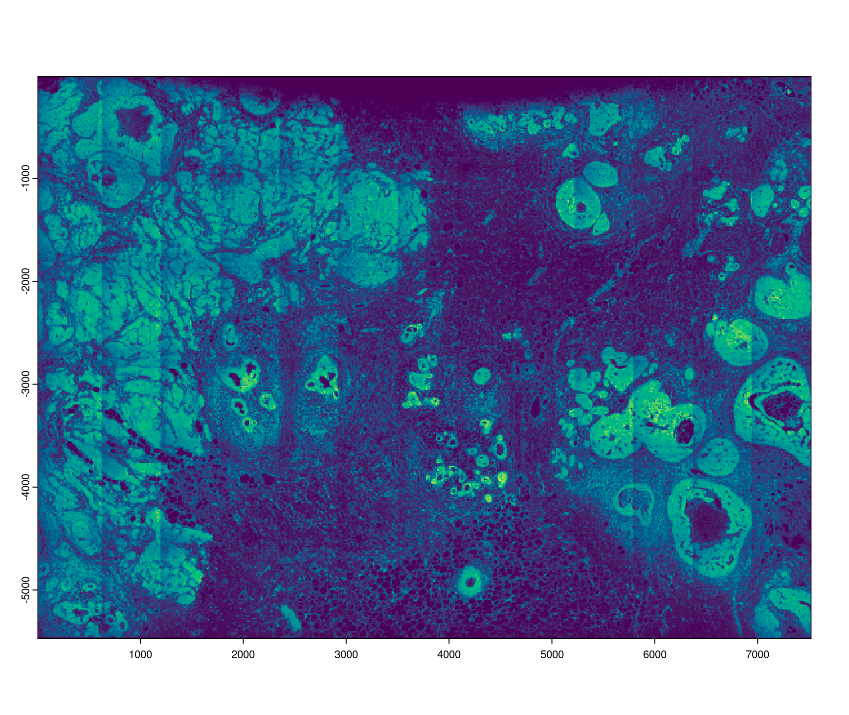
plot of Gene expression (rna) density
#   [1] "ABCC11"   "ACTA2"    "ACTG2"    "ADAM9"    "ADGRE5"   "ADH1B"
#   [7] "ADIPOQ"   "AGR3"     "AHSP"     "AIF1"     "AKR1C1"   "AKR1C3"
#  [13] "ALDH1A3"  "ANGPT2"   "ANKRD28"  "ANKRD29"  "ANKRD30A" "APOBEC3A"
#  [19] "APOBEC3B" "APOC1"    "AQP1"     "AQP3"     "AR"       "AVPR1A"
#  [25] "BACE2"    "BANK1"    "BASP1"    "BTNL9"    "C15orf48" "C1QA"
#  [31] "C1QC"     "C2orf42"  "C5orf46"  "C6orf132" "CAV1"     "CAVIN2"
#  [37] "CCDC6"    "CCDC80"   "CCL20"    "CCL5"     "CCL8"     "CCND1"
#  [43] "CCPG1"    "CCR7"     "CD14"     "CD163"    "CD19"     "CD1C"
#  [49] "CD247"    "CD27"     "CD274"    "CD3D"     "CD3E"     "CD3G"
#  [55] "CD4"      "CD68"     "CD69"     "CD79A"    "CD79B"    "CD80"
#  [61] "CD83"     "CD86"     "CD8A"     "CD8B"     "CD9"      "CD93"
#  [67] "CDC42EP1" "CDH1"     "CEACAM6"  "CEACAM8"  "CENPF"    "CLCA2"
#  [73] "CLDN4"    "CLDN5"    "CLEC14A"  "CLEC9A"   "CLECL1"   "CLIC6"
#  [79] "CPA3"     "CRHBP"    "CRISPLD2" "CSF3"     "CTH"      "CTLA4"
#  [85] "CTSG"     "CTTN"     "CX3CR1"   "CXCL12"   "CXCL16"   "CXCL5"
#  [91] "CXCR4"    "CYP1A1"   "CYTIP"    "DAPK3"    "DERL3"    "DMKN"
#  [97] "DNAAF1"   "DNTTIP1"  "DPT"      "DSC2"     "DSP"      "DST"
# [103] "DUSP2"    "DUSP5"    "EDN1"     "EDNRB"    "EGFL7"    "EGFR"
# [109] "EIF4EBP1" "ELF3"     "ELF5"     "ENAH"     "EPCAM"    "ERBB2"
# [115] "ERN1"     "ESM1"     "ESR1"     "FAM107B"  "FAM49A"   "FASN"
# [121] "FBLIM1"   "FBLN1"    "FCER1A"   "FCER1G"   "FCGR3A"   "FGL2"
# [127] "FLNB"     "FOXA1"    "FOXC2"    "FOXP3"    "FSTL3"    "GATA3"
# [133] "GJB2"     "GLIPR1"   "GNLY"     "GPR183"   "GZMA"     "GZMB"
# [139] "GZMK"     "HAVCR2"   "HDC"      "HMGA1"    "HOOK2"    "HOXD8"
# [145] "HOXD9"    "HPX"      "IGF1"     "IGSF6"    "IL2RA"    "IL2RG"
# [151] "IL3RA"    "IL7R"     "ITGAM"    "ITGAX"    "ITM2C"    "JUP"
# [157] "KARS"     "KDR"      "KIT"      "KLF5"     "KLRB1"    "KLRC1"
# [163] "KLRD1"    "KLRF1"    "KRT14"    "KRT15"    "KRT16"    "KRT23"
# [169] "KRT5"     "KRT6B"    "KRT7"     "KRT8"     "LAG3"     "LARS"
# [175] "LDHB"     "LEP"      "LGALSL"   "LIF"      "LILRA4"   "LPL"
# [181] "LPXN"     "LRRC15"   "LTB"      "LUM"      "LY86"     "LYPD3"
# [187] "LYZ"      "MAP3K8"   "MDM2"     "MEDAG"    "MKI67"    "MLPH"
# [193] "MMP1"     "MMP12"    "MMP2"     "MMRN2"    "MNDA"     "MPO"
# [199] "MRC1"     "MS4A1"    "MUC6"     "MYBPC1"   "MYH11"    "MYLK"
# [205] "MYO5B"    "MZB1"     "NARS"     "NCAM1"    "NDUFA4L2" "NKG7"
# [211] "NOSTRIN"  "NPM3"     "OCIAD2"   "OPRPN"    "OXTR"     "PCLAF"
# [217] "PCOLCE"   "PDCD1"    "PDCD1LG2" "PDE4A"    "PDGFRA"   "PDGFRB"
# [223] "PDK4"     "PECAM1"   "PELI1"    "PGR"      "PIGR"     "PIM1"
# [229] "PLD4"     "POLR2J3"  "POSTN"    "PPARG"    "PRDM1"    "PRF1"
# [235] "PTGDS"    "PTN"      "PTPRC"    "PTRHD1"   "QARS"     "RAB30"
# [241] "RAMP2"    "RAPGEF3"  "REXO4"    "RHOH"     "RORC"     "RTKN2"
# [247] "RUNX1"    "S100A14"  "S100A4"   "S100A8"   "SCD"      "SCGB2A1"
# [253] "SDC4"     "SEC11C"   "SEC24A"   "SELL"     "SERHL2"   "SERPINA3"
# [259] "SERPINB9" "SFRP1"    "SFRP4"    "SH3YL1"   "SLAMF1"   "SLAMF7"
# [265] "SLC25A37" "SLC4A1"   "SLC5A6"   "SMAP2"    "SMS"      "SNAI1"
# [271] "SOX17"    "SOX18"    "SPIB"     "SQLE"     "SRPK1"    "SSTR2"
# [277] "STC1"     "SVIL"     "TAC1"     "TACSTD2"  "TCEAL7"   "TCF15"
# [283] "TCF4"     "TCF7"     "TCIM"     "TCL1A"    "TENT5C"   "TFAP2A"
# [289] "THAP2"    "TIFA"     "TIGIT"    "TIMP4"    "TMEM147"  "TNFRSF17"
# [295] "TOMM7"    "TOP2A"    "TPD52"    "TPSAB1"   "TRAC"     "TRAF4"
# [301] "TRAPPC3"  "TRIB1"    "TUBA4A"   "TUBB2B"   "TYROBP"   "UCP1"
# [307] "USP53"    "VOPP1"    "VWF"      "WARS"     "ZEB1"     "ZEB2"
# [313] "ZNF562"
Blank Codeword (159) - (QC) Codewords that should not be used in the current panel. (named Unassigned Codeword in later Xenium pipelines)
#   [1] "BLANK_0006" "BLANK_0013" "BLANK_0037" "BLANK_0069" "BLANK_0072"
#   [6] "BLANK_0087" "BLANK_0110" "BLANK_0114" "BLANK_0120" "BLANK_0147"
#  [11] "BLANK_0180" "BLANK_0186" "BLANK_0272" "BLANK_0278" "BLANK_0319"
#  [16] "BLANK_0321" "BLANK_0337" "BLANK_0350" "BLANK_0351" "BLANK_0352"
#  [21] "BLANK_0353" "BLANK_0354" "BLANK_0355" "BLANK_0356" "BLANK_0357"
#  [26] "BLANK_0358" "BLANK_0359" "BLANK_0360" "BLANK_0361" "BLANK_0362"
#  [31] "BLANK_0363" "BLANK_0364" "BLANK_0365" "BLANK_0366" "BLANK_0367"
#  [36] "BLANK_0368" "BLANK_0369" "BLANK_0370" "BLANK_0371" "BLANK_0372"
#  [41] "BLANK_0373" "BLANK_0374" "BLANK_0375" "BLANK_0376" "BLANK_0377"
#  [46] "BLANK_0378" "BLANK_0379" "BLANK_0380" "BLANK_0381" "BLANK_0382"
#  [51] "BLANK_0383" "BLANK_0384" "BLANK_0385" "BLANK_0386" "BLANK_0387"
#  [56] "BLANK_0388" "BLANK_0389" "BLANK_0390" "BLANK_0391" "BLANK_0392"
#  [61] "BLANK_0393" "BLANK_0394" "BLANK_0395" "BLANK_0396" "BLANK_0397"
#  [66] "BLANK_0398" "BLANK_0399" "BLANK_0400" "BLANK_0401" "BLANK_0402"
#  [71] "BLANK_0403" "BLANK_0404" "BLANK_0405" "BLANK_0406" "BLANK_0407"
#  [76] "BLANK_0408" "BLANK_0409" "BLANK_0410" "BLANK_0411" "BLANK_0412"
#  [81] "BLANK_0413" "BLANK_0414" "BLANK_0415" "BLANK_0416" "BLANK_0417"
#  [86] "BLANK_0418" "BLANK_0419" "BLANK_0420" "BLANK_0421" "BLANK_0422"
#  [91] "BLANK_0423" "BLANK_0424" "BLANK_0425" "BLANK_0426" "BLANK_0427"
#  [96] "BLANK_0428" "BLANK_0429" "BLANK_0430" "BLANK_0431" "BLANK_0432"
# [101] "BLANK_0433" "BLANK_0434" "BLANK_0435" "BLANK_0436" "BLANK_0437"
# [106] "BLANK_0438" "BLANK_0439" "BLANK_0440" "BLANK_0441" "BLANK_0442"
# [111] "BLANK_0443" "BLANK_0444" "BLANK_0445" "BLANK_0446" "BLANK_0447"
# [116] "BLANK_0448" "BLANK_0449" "BLANK_0450" "BLANK_0451" "BLANK_0452"
# [121] "BLANK_0453" "BLANK_0454" "BLANK_0455" "BLANK_0456" "BLANK_0457"
# [126] "BLANK_0458" "BLANK_0459" "BLANK_0460" "BLANK_0461" "BLANK_0462"
# [131] "BLANK_0463" "BLANK_0464" "BLANK_0465" "BLANK_0466" "BLANK_0467"
# [136] "BLANK_0468" "BLANK_0469" "BLANK_0470" "BLANK_0471" "BLANK_0472"
# [141] "BLANK_0473" "BLANK_0474" "BLANK_0475" "BLANK_0476" "BLANK_0477"
# [146] "BLANK_0478" "BLANK_0479" "BLANK_0480" "BLANK_0481" "BLANK_0482"
# [151] "BLANK_0483" "BLANK_0484" "BLANK_0485" "BLANK_0486" "BLANK_0487"
# [156] "BLANK_0488" "BLANK_0489" "BLANK_0497" "BLANK_0499"
Negative Control Codeword (41) - (QC) Codewords that do not map to genes, but are in the codebook. Used to determine specificity of decoding algorithm
#  [1] "NegControlCodeword_0500" "NegControlCodeword_0501"
#  [3] "NegControlCodeword_0502" "NegControlCodeword_0503"
#  [5] "NegControlCodeword_0504" "NegControlCodeword_0505"
#  [7] "NegControlCodeword_0506" "NegControlCodeword_0507"
#  [9] "NegControlCodeword_0508" "NegControlCodeword_0509"
# [11] "NegControlCodeword_0510" "NegControlCodeword_0511"
# [13] "NegControlCodeword_0512" "NegControlCodeword_0513"
# [15] "NegControlCodeword_0514" "NegControlCodeword_0515"
# [17] "NegControlCodeword_0516" "NegControlCodeword_0517"
# [19] "NegControlCodeword_0518" "NegControlCodeword_0519"
# [21] "NegControlCodeword_0520" "NegControlCodeword_0521"
# [23] "NegControlCodeword_0522" "NegControlCodeword_0523"
# [25] "NegControlCodeword_0524" "NegControlCodeword_0525"
# [27] "NegControlCodeword_0526" "NegControlCodeword_0527"
# [29] "NegControlCodeword_0528" "NegControlCodeword_0529"
# [31] "NegControlCodeword_0530" "NegControlCodeword_0531"
# [33] "NegControlCodeword_0532" "NegControlCodeword_0533"
# [35] "NegControlCodeword_0534" "NegControlCodeword_0535"
# [37] "NegControlCodeword_0536" "NegControlCodeword_0537"
# [39] "NegControlCodeword_0538" "NegControlCodeword_0539"
# [41] "NegControlCodeword_0540"
Negative Control Probe (28) - (QC) Probes in panel but target non-biological sequences. Used to determine specificity of assay.
#  [1] "NegControlProbe_00042" "NegControlProbe_00041" "NegControlProbe_00039"
#  [4] "NegControlProbe_00035" "NegControlProbe_00034" "NegControlProbe_00033"
#  [7] "NegControlProbe_00031" "NegControlProbe_00025" "NegControlProbe_00024"
# [10] "NegControlProbe_00022" "NegControlProbe_00019" "NegControlProbe_00017"
# [13] "NegControlProbe_00016" "NegControlProbe_00014" "NegControlProbe_00013"
# [16] "NegControlProbe_00012" "NegControlProbe_00009" "NegControlProbe_00004"
# [19] "NegControlProbe_00003" "NegControlProbe_00002" "antisense_PROKR2"
# [22] "antisense_ULK3"        "antisense_SCRIB"       "antisense_TRMU"
# [25] "antisense_MYLIP"       "antisense_LGI3"        "antisense_BCL2L15"
# [28] "antisense_ADCY4"
The main thing to watch out for is that the other probe types should be separated out from the the Gene expression or rna feature type so that they do not interfere with expression normalization and other analyses.
How to deal with these different types of detections is easily
adjustable. With the feat_type param you declare which
categories/feat_types you want to split transcript
detections into. Then with split_keyword, you provide a
list of character vectors containing grep() terms to search
for.
Note that there are 4 feat_types declared in this set of
defaults, but 3 items passed to split_keyword. Any
transcripts not matched by items in split_keyword, get
categorized as the first provided feat_type (“rna”).
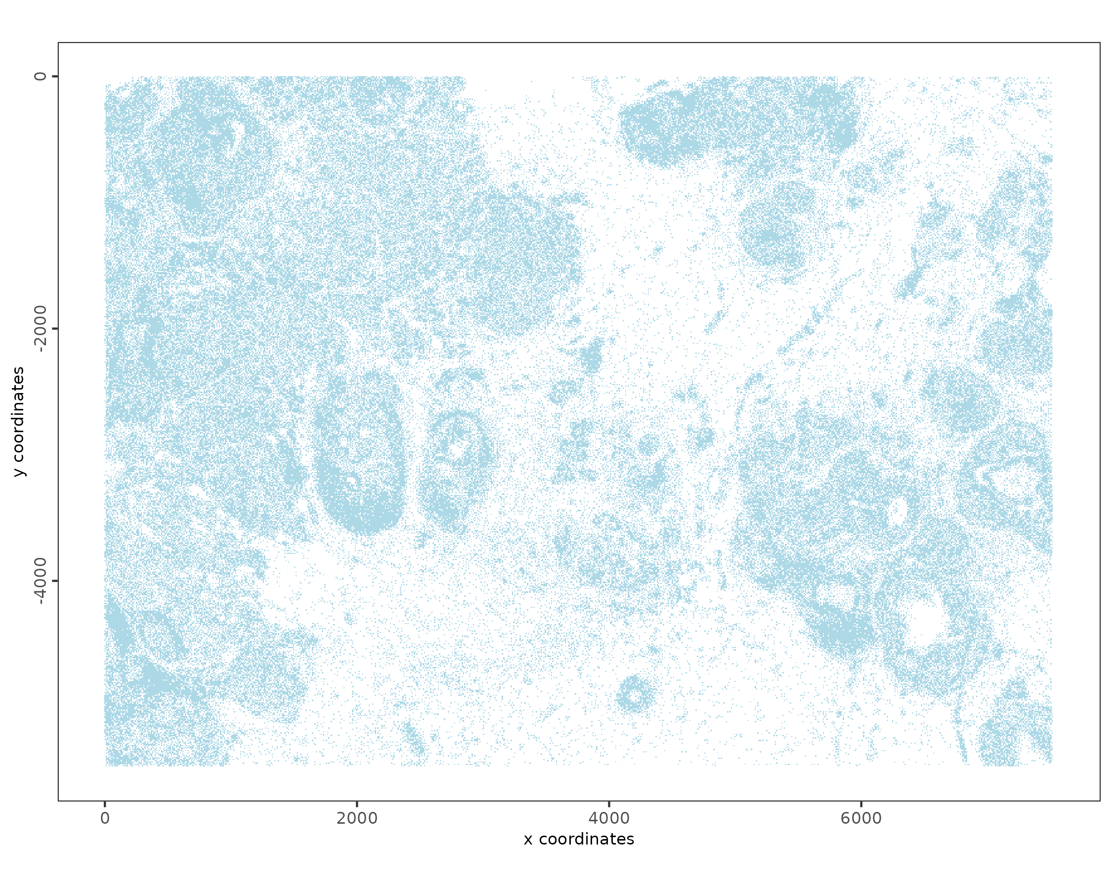
# Example plot
spatPlot2D(xenium_gobj,
    # scattermore speeds up plotting
    plot_method = "scattermore",
    point_shape = "no_border",
    point_size = 1
)
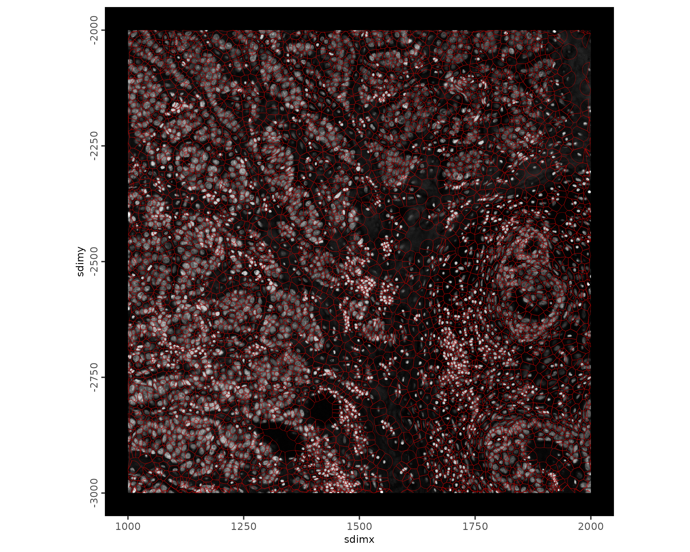
# zoomed in region with polygons and image
spatInSituPlotPoints(xenium_gobj,
    show_image = TRUE,
    polygon_line_size = 0.1,
    polygon_color = "#BB0000",
    polygon_alpha = 0.2,
    xlim = c(1000, 2000),
    ylim = c(-3000, -2000)
)
3.1 Attaching Post-Xenium Aligned Images (Optional)
Xenium runs will come with one or more IF morphology images. In this dataset, it is just the DAPI image. Additional images of the tissue generated after the Xenium run can be added by aligning new images to the rest of the Xenium information. These alignments are provided as affine matrices.
Here we will load in the post-Xenium H&E and IF images.
The images used in this process are ome.tif images which
Giotto is not fully compatible with, so we convert any images we will
use to normal tif images using
ometif_to_tif().
This image format conversion is a step that is automatically done with the morphology images.
# image conversions
path_he <- "path/to/...he_image.ome.tif"
path_if <- "path/to/...if_image.ome.tif"

# conversion `output_dir` can be specified
# default is a new subdirectory called `tif_exports`
conv_path_he <- GiottoClass::ometif_to_tif(path_he)

# IF staining is a 3 page .ome.tif
conv_path_if <- lapply(1:3, function(p) {
    GiottoClass::ometif_to_tif(path_if, page = p)
})

# with the following channel names
# 1. CD20, 2. HER2, 3. DAPI
if_channels <- GiottoClass::ometif_metadata(path_if, node = "Channel")$Name

# use the `importXenium()` custom loading utility
x <- importXenium(file.path(data_path, "outs"))

img_he <- x$load_aligned_image(
    name = "post_he",
    path = conv_path_he, # "path/to/tif_exports/...he_image.tif"
    imagealignment_path = "path/to/...he_imagealignment.csv"
)
img_if <- lapply(1:3, function(if_i) {
    x$load_aligned_image(
        name = if_channels[[if_i]],
        path = conv_path_if[[if_i]], # "path/to/tif_exports/...if_image.tif"
        imagealignment_path = "path/to/...if_imagealignment.csv"
    )
})

plot(img_he)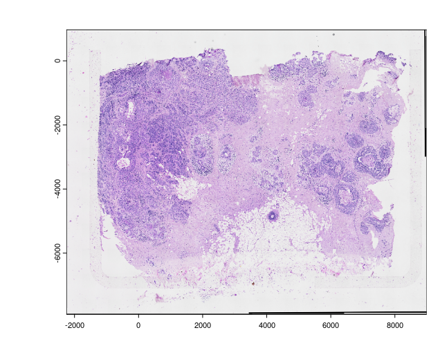
plot(img_if[[2]])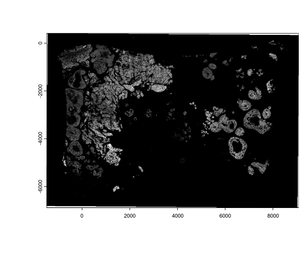
# append to giotto object
xenium_gobj <- setGiotto(xenium_gobj, c(list(img_he), img_if))

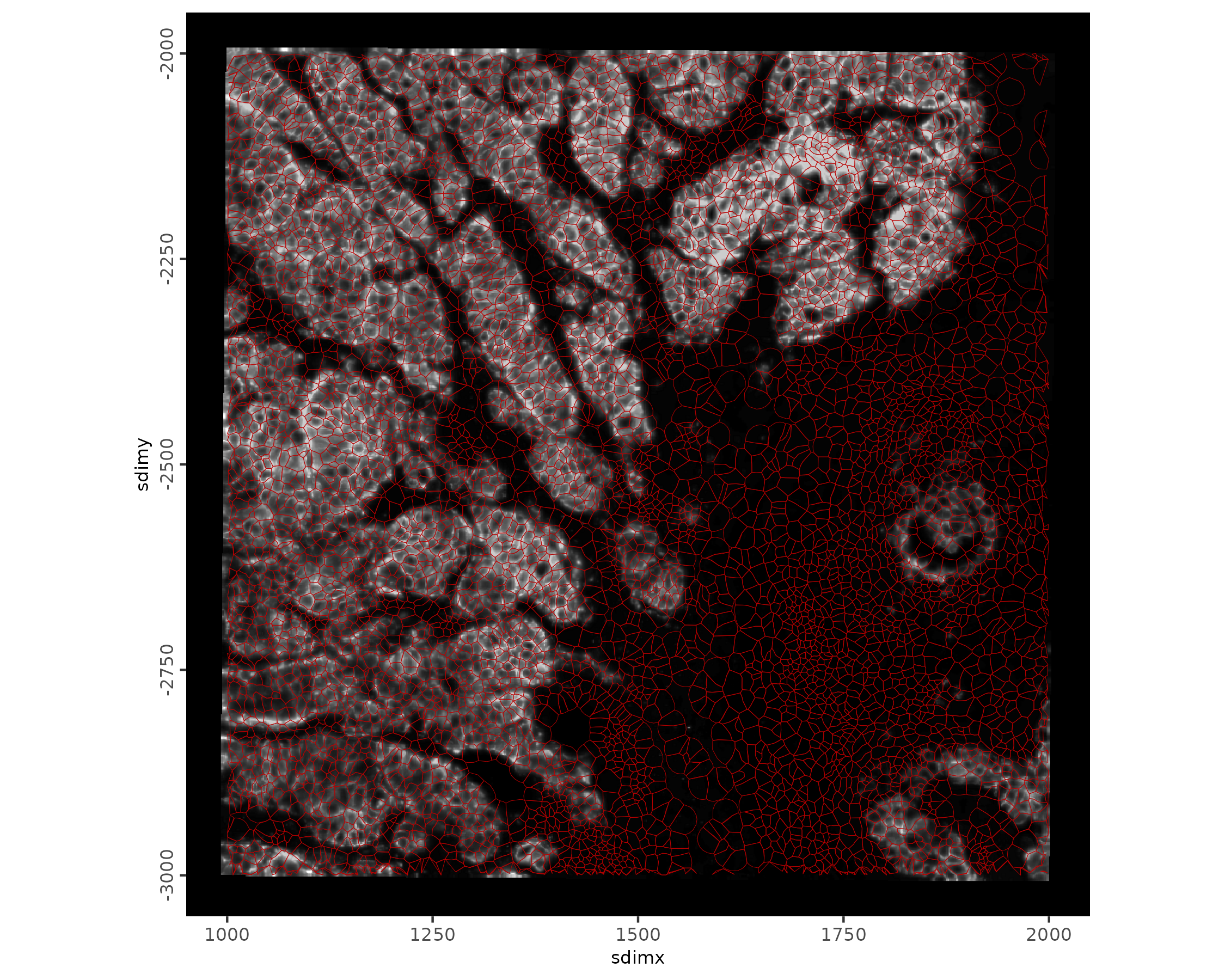
# example plot with HER2
spatInSituPlotPoints(xenium_gobj,
    xlim = c(1000, 2000),
    ylim = c(-3000, -2000),
    show_image = TRUE,
    image_name = "HER2",
    polygon_line_size = 0.1,
    polygon_color = "#BB0000",
    polygon_alpha = 0.2
)
4 Aggregate Data
# Calculate Overlaps of `"rna"` Features with the `"cell"` Polygon Boundaries
xenium_gobj <- calculateOverlapRaster(xenium_gobj,
    spatial_info = 'cell',
    feat_info = 'rna'
)

# Assign polygon overlaps information to expression matrix
xenium_gobj <- overlapToMatrix(xenium_gobj,
    poly_info = 'cell',
    feat_info = 'rna',
    name = 'raw'
)

showGiottoExpression(xenium_gobj)
└──Spatial unit "cell"
└──Feature type "rna"
└──Expression data "raw" values:
An object of class exprObj : "raw"
spat_unit : "cell"
feat_type : "rna"
provenance: cell
contains:
313 x 167780 sparse Matrix of class "dgCMatrix"
ABCC11 . . . . . . . . . . . . . ......
ACTA2 . . . . . . . 1 . . . . 1 ......
ACTG2 . 2 . . . . 1 . . . . . 1 ......
........suppressing 167767 columns and 307 rows in show()
ZEB1 . . . . . . . . . 1 . . . ......
ZEB2 . . . . . 2 . . 2 1 1 . . ......
ZNF562 . . . . . . . . . . . . . ......
First four colnames:
1 2 3 4 This is now a fully functioning Xenium giotto object.
From here, we can do the standard data processing pipeline to
cluster.
5 Data Processing
Now that an aggregated expression matrix is generated, the usual data filtering and processing can be applied We start by setting a count of 1 to be the minimum to consider a feature expressed. A feature must be detected in at least 3 cells to be included. Lastly, a cell must have a minimum of 5 features detected to be included.
# process the data up to PCA calculation
xenium_gobj <- xenium_gobj |>
    filterGiotto(,
        spat_unit = 'cell',
        expression_threshold = 1,
        feat_det_in_min_cells = 3,
        min_det_feats_per_cell = 5
    ) |>
    normalizeGiotto() |>
    addStatistics() |>
    runPCA(feats_to_use = NULL) # don't use HVFs since there are too few features*
**By default, runPCA() uses the subset of genes
discovered to be highly variable and then assigned as such in the
feature metadata. Instead, this time, using all genes is desireable, so
feats_to_use will be set to NULL.*
# Visualize Screeplot and PCA
screePlot(xenium_gobj, ncp = 20)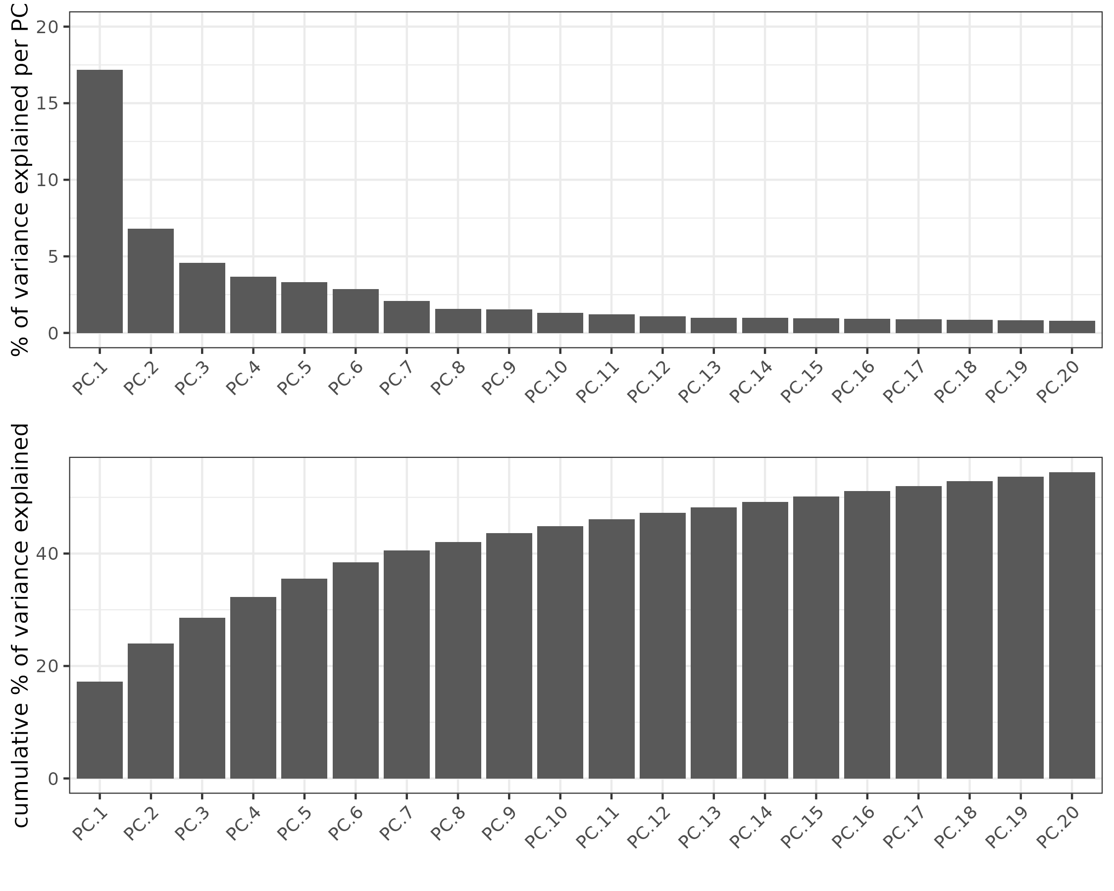
plotPCA(xenium_gobj, point_size = 0.1)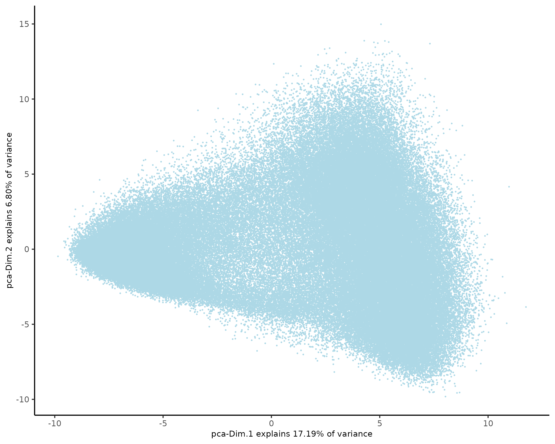
5.1 Dimension Reduction
xenium_gobj = runtSNE(xenium_gobj, dimensions_to_use = 1:10)
xenium_gobj = runUMAP(xenium_gobj, dimensions_to_use = 1:10)

plotTSNE(xenium_gobj, point_size = 0.01)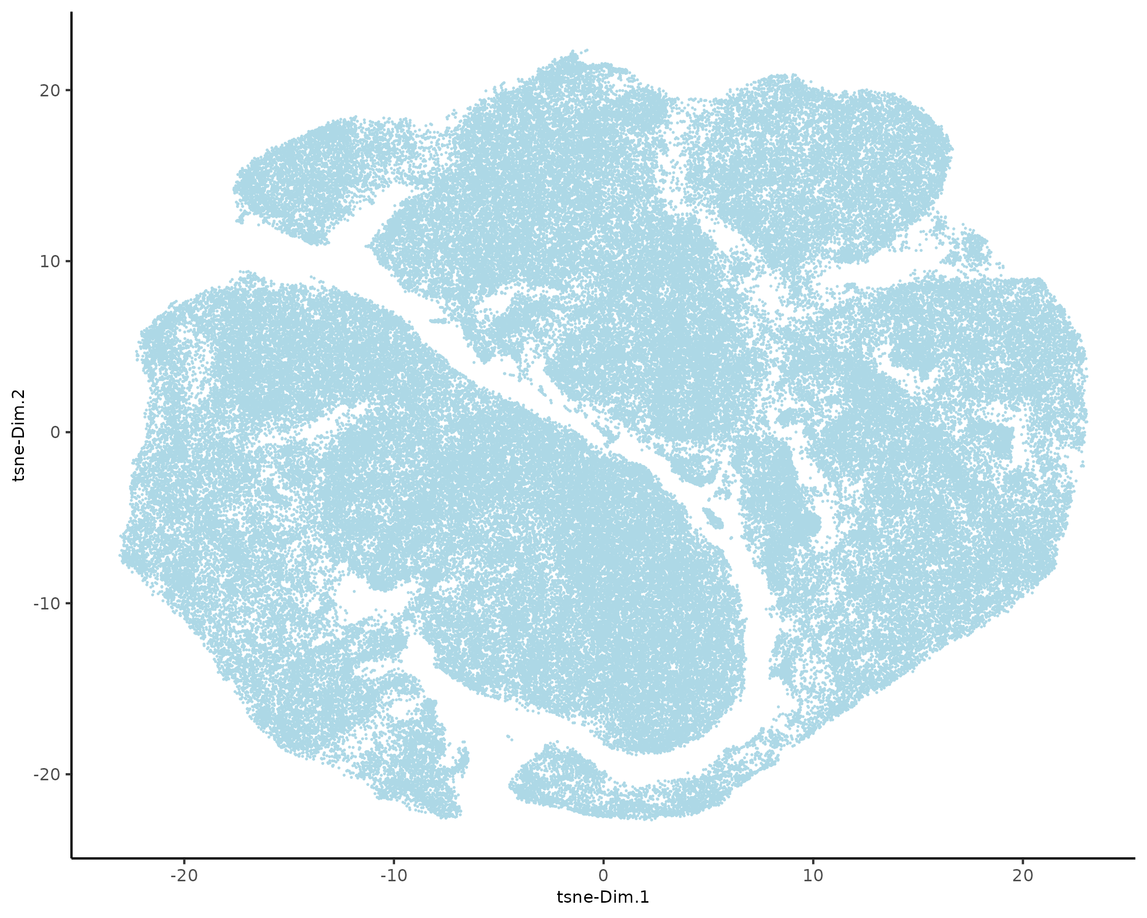
plotUMAP(xenium_gobj, point_size = 0.01)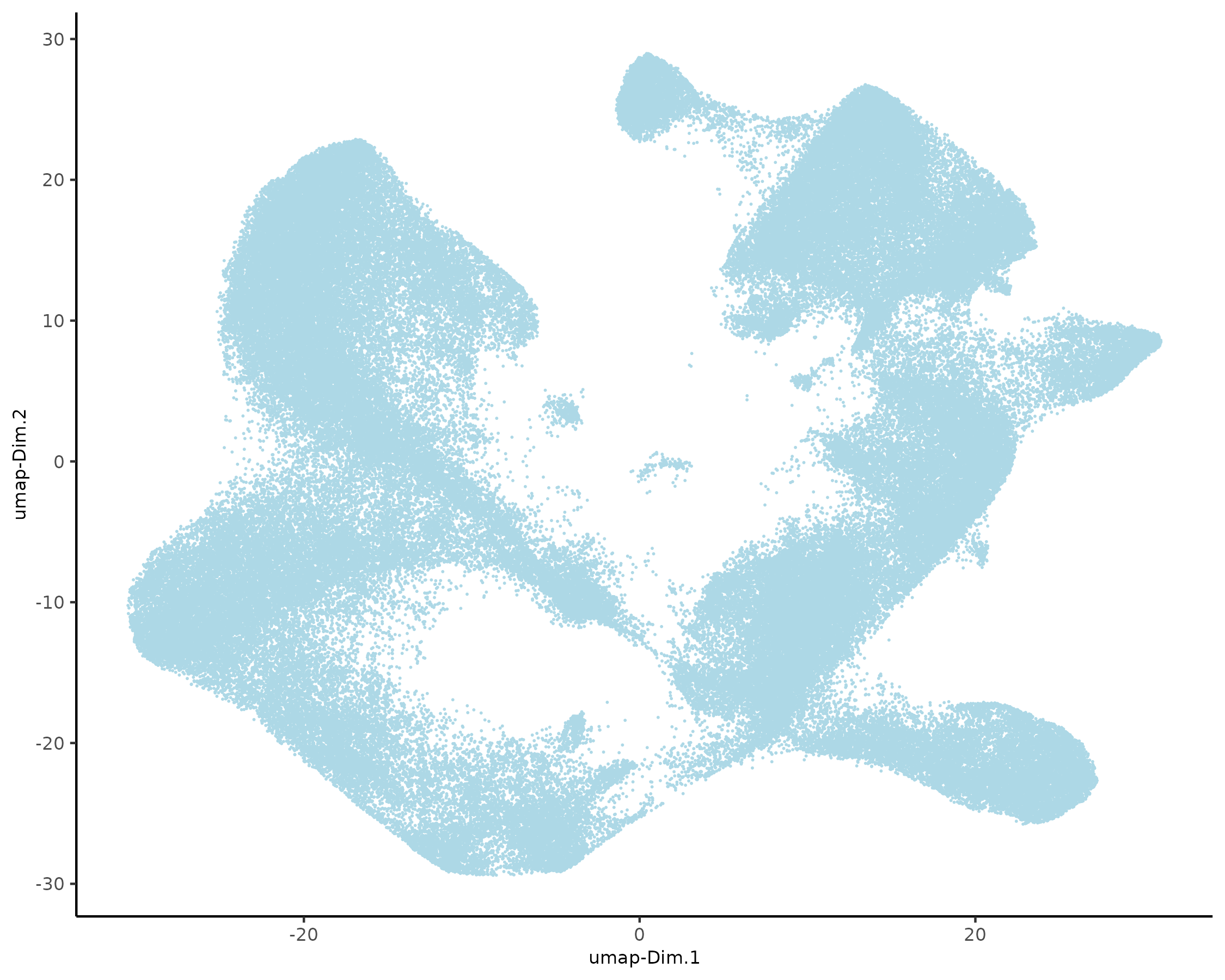
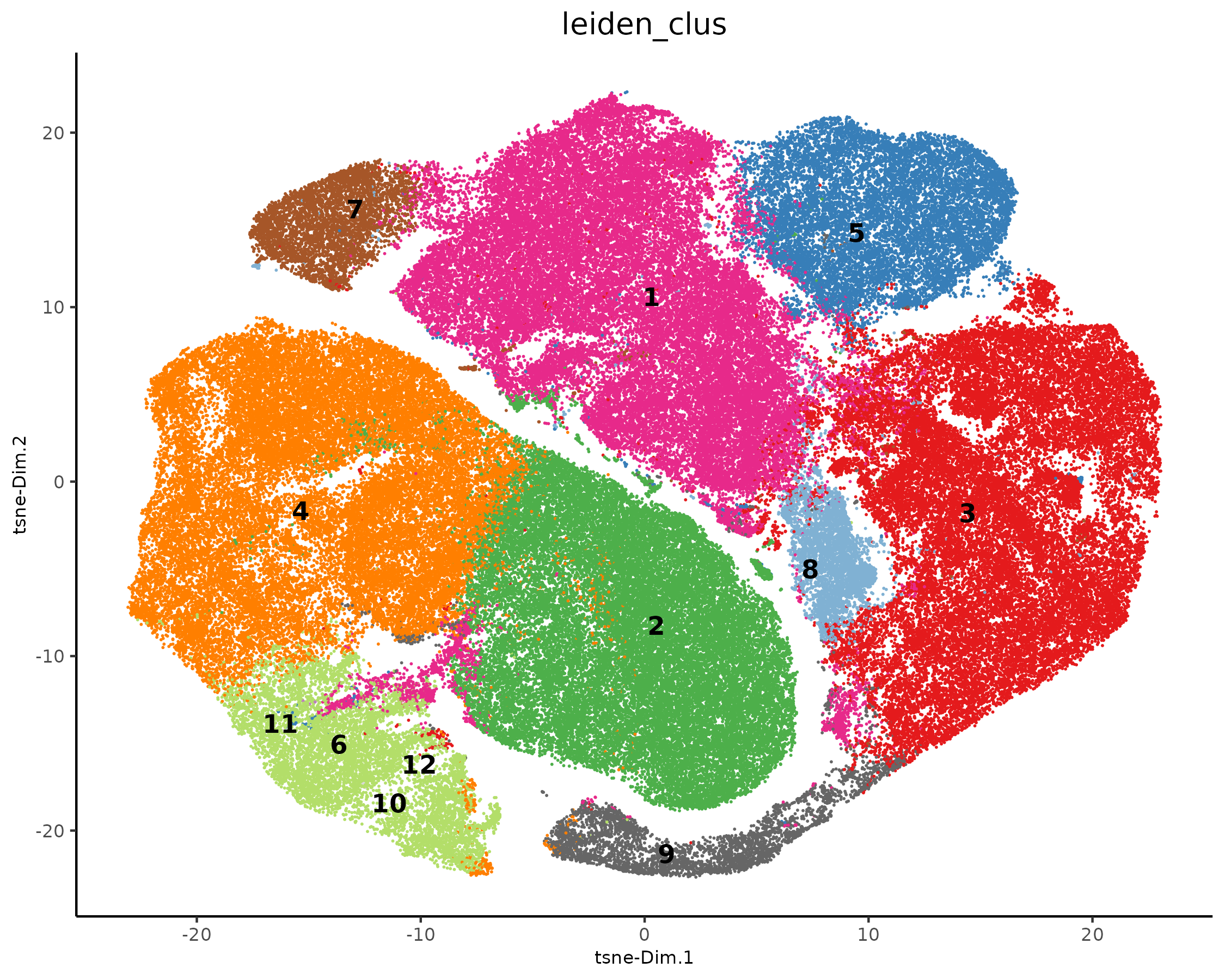
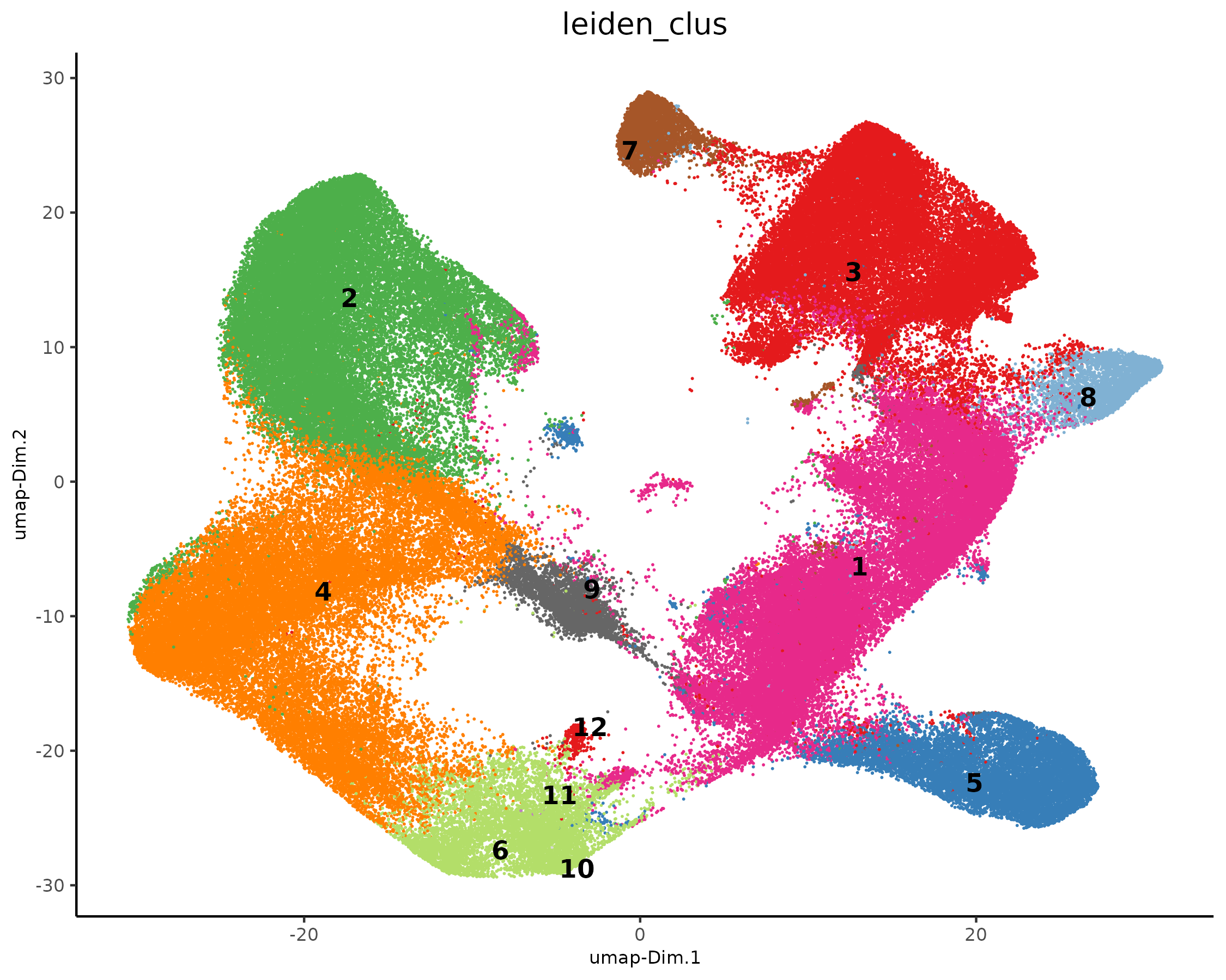
5.2 Clustering
# create Shared Nearest Neighbors Network
xenium_gobj <- xenium_gobj |>
        createNearestNetwork(dimensions_to_use = 1:10, k = 10) |>
        doLeidenCluster(resolution = 0.25, n_iterations = 100)

# visualize UMAP cluster results
plotTSNE(xenium_gobj,
    cell_color = 'leiden_clus',
    show_legend = FALSE,
    point_size = 0.01,
    point_shape = 'no_border'
)
plotUMAP(xenium_gobj,
    cell_color = 'leiden_clus',
    show_legend = FALSE,
    point_size = 0.01,
    point_shape = 'no_border'
)
5.3 Visualize UMAP and Spatial Results
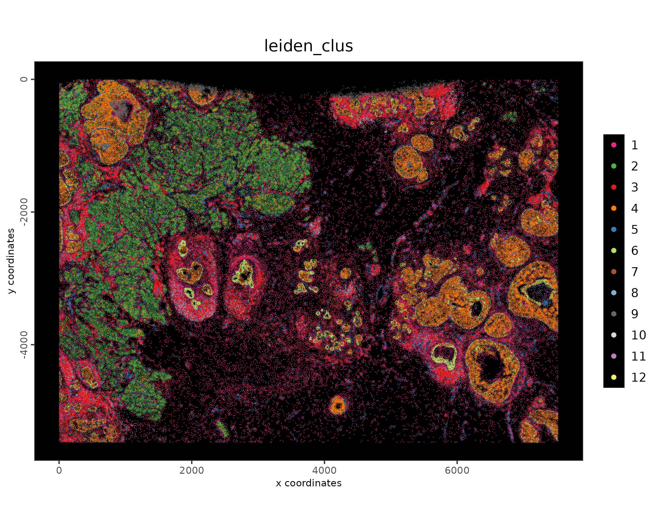
# centroids plotting
spatPlot2D(xenium_gobj,
    plot_method = "scattermore",
    cell_color = 'leiden_clus',
    point_size = 0.1,
    point_shape = 'no_border',
    background_color = 'black'
)
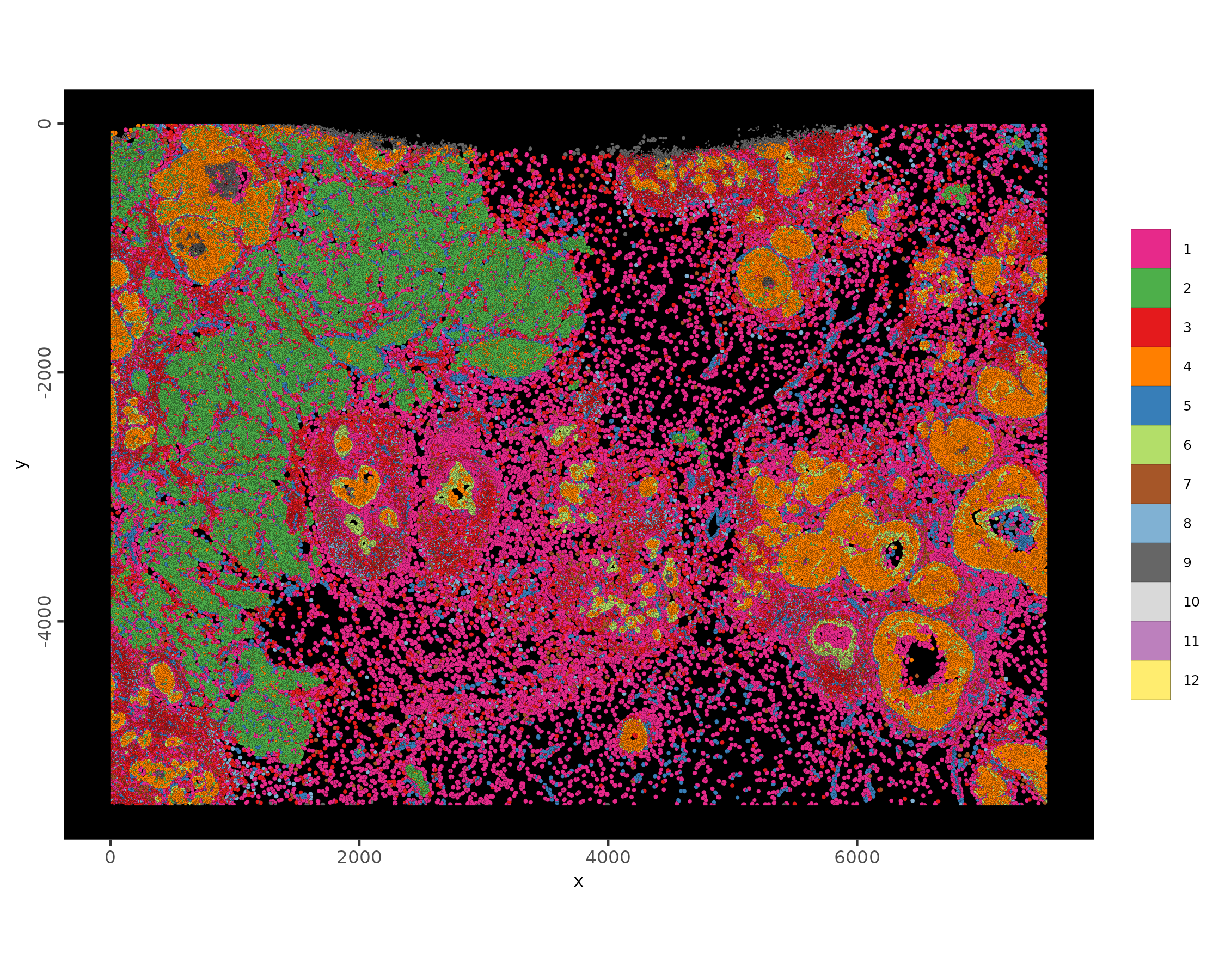
5.4 Subcellular Visualization
# plot with polygons
spatInSituPlotPoints(xenium_gobj,
    polygon_feat_type = 'cell',
    polygon_alpha = 1,
    polygon_line_size = 0.01,
    polygon_color = 'black',
    polygon_fill = 'leiden_clus',
    polygon_fill_as_factor = TRUE
)
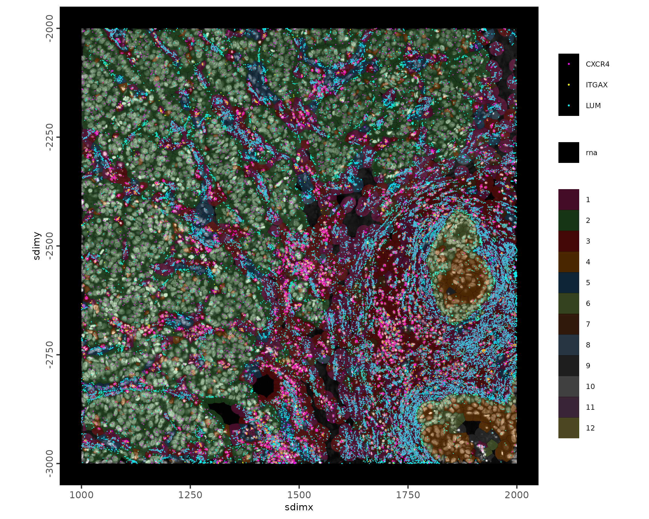
# visualize with points in a spatial subset
spatInSituPlotPoints(xenium_gobj,
    feats = list('rna' = c(
        "LUM", "CXCR4", "ITGAX"
    )),
    feats_color_code = c(
        "LUM" = 'cyan',
        'CXCR4' = 'magenta',
        'ITGAX' = 'yellow'
    ),
    point_size = 0.1,
    xlim = c(1000, 2000),
    ylim = c(-3000, -2000),
    plot_last = "polygons",
    polygon_feat_type = 'cell',
    polygon_alpha = 0.3,
    polygon_line_size = 0.01,
    polygon_color = 'black',
    polygon_fill = 'leiden_clus',
    polygon_fill_as_factor = TRUE,
    show_image = TRUE,
    image_name = "dapi"
)
5.5 Visualize Known Markers
dimFeatPlot2D(xenium_gobj,
    feats = c(
        "CD3E", "CD8A", "CD4", # T cell
        "JCHAIN", # plasmablast
        "MS4A1", # B
        "DCN", "SFRP2", # CAF (mesenchymal)
        "TAGLN", # CAF/PVL (mesenchymal)
        "RAMP2", # endothelial
        "PROX1", # LEC (lymphatic endothelial cell)
        "TYROBP", # myeloid
        "CPA3", "TPSAB1", # mast cell
        "SPINT2", "MKI67", "KRT8", # epithelial/cancer
        "SOX10", "TP63", # myoepithelial
        "CD24", # B cell and cancer stemness
        "PDCD1" # PD1
    ),
    point_size = 0.2,
    point_border_stroke = 0,
    background_color = "black",
    cow_n_col = 4,
    show_legend = FALSE,
    gradient_style = "sequential",
    save_param = list(
      "base_height" = 6
    )
)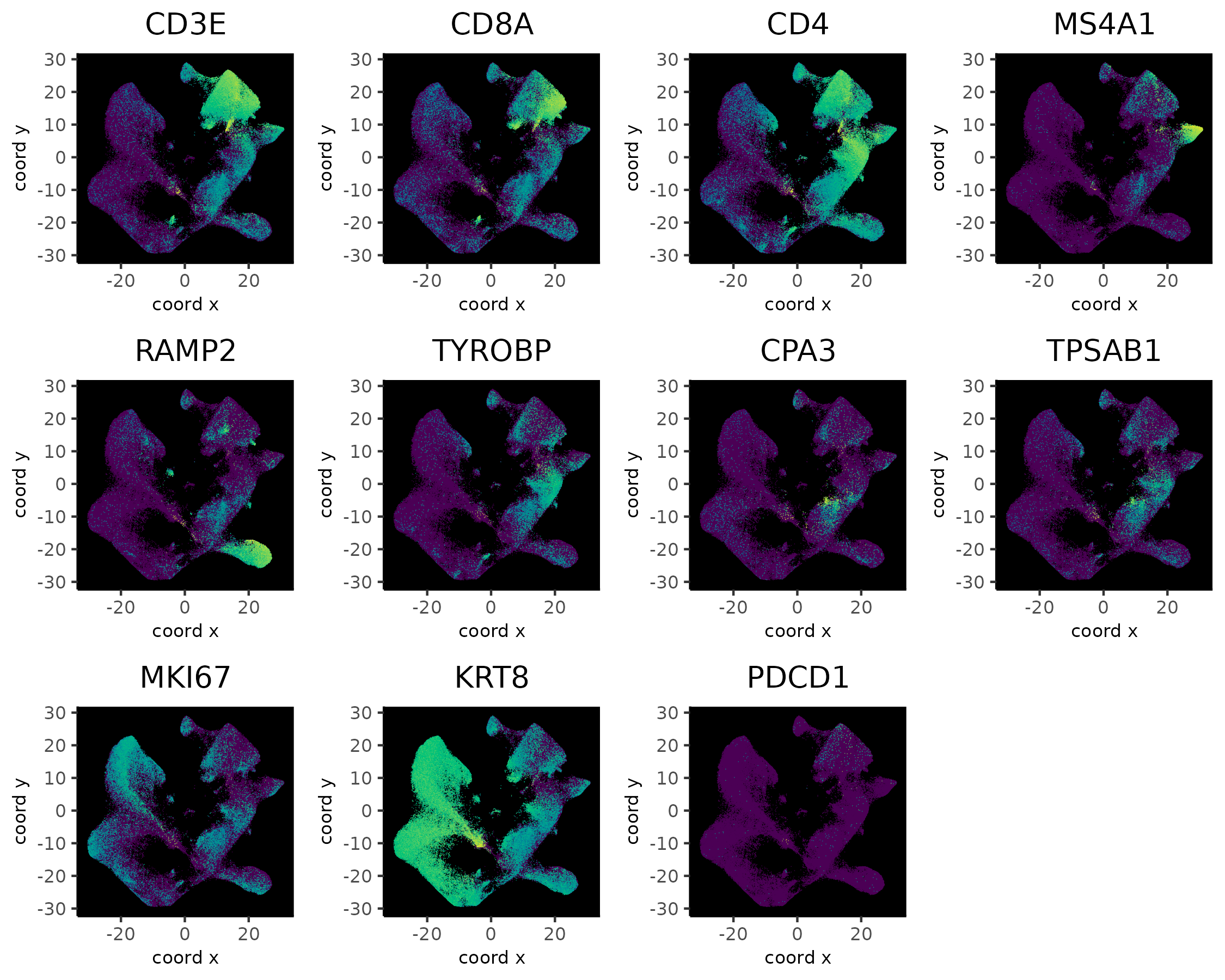
These markers are not very specific to the UMAP clustering. Several genes were also not available in the panel.
6 Single Cell Assisted Cell Typing
Xenium datasets have very sensitive target detection, but
segmentation plays a large role in how clean the expression information
is. This dataset did not come with bound staining segmentation and the
'cell' segmentation is instead a simple expansion-based
approach performed on top of the 'nucleus' annotations. As
a result, many transcripts may be assigned to the wrong cell.
Single cell datasets lack spatial context, however they tend to have clearer separation between clusters, making it easier to see which clusters correspond to which cell types. This dataset comes with paired single cell datasets at GSE243280. We can use the single cell data to cell type, then transfer those labels to the Xenium data.
More specifically, we will be using the 5 prime dataset GSM7782696.
6.1 Single Cell Processing
First we need to process the single cell dataset and cell type it.
single cell data processing
Load Single Cell Data
expr_data_path <- "path/to/5p_count_filtered_feature_bc_matrix.h5"
# create single cell giotto object
sc <- createGiottoObject(
    expression = get10Xmatrix_h5(expr_data_path)$`Gene Expression`,
    instructions = instrs
)
Pre-Process: Mitochondrial Filtering
fids <- featIDs(sc)
mt_genes <- fids[grep("^MT-.*", fids)]
sc <- addFeatsPerc(sc, expression_values = "raw", feats = mt_genes, vector_name = "mito")

library(ggplot2)
ggplot(spatValues(sc, feats = "mito"), aes(x = "cells", y = mito)) + geom_violin()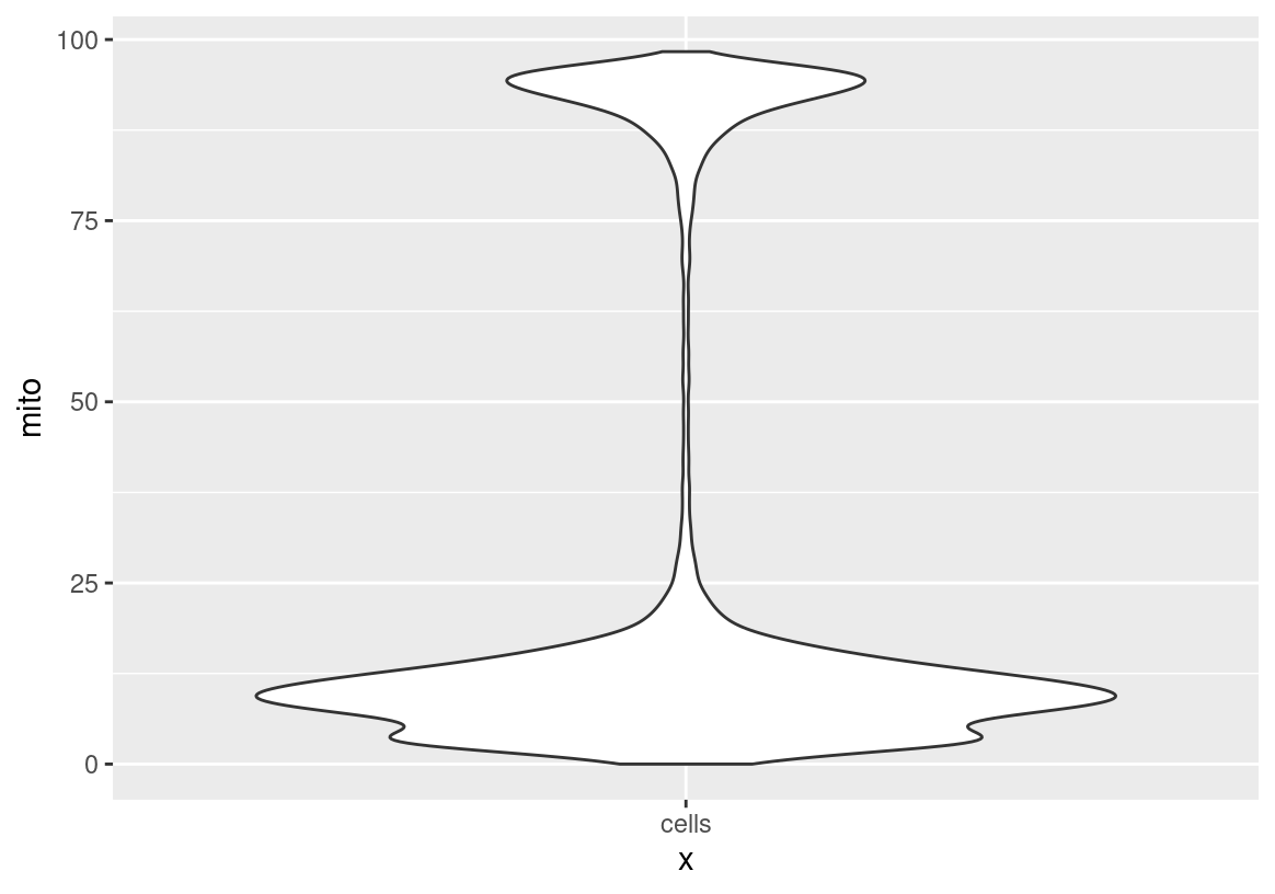
meta <- pDataDT(sc)
meta[, sum(mito > 50)] # 5006 # filter these out
meta[, sum(mito < 50)] # 17963
sc <- subset(sc, subset = mito < 50)
ggplot(spatValues(sc, feats = "mito"), aes(x = "cells", y = mito)) + geom_violin()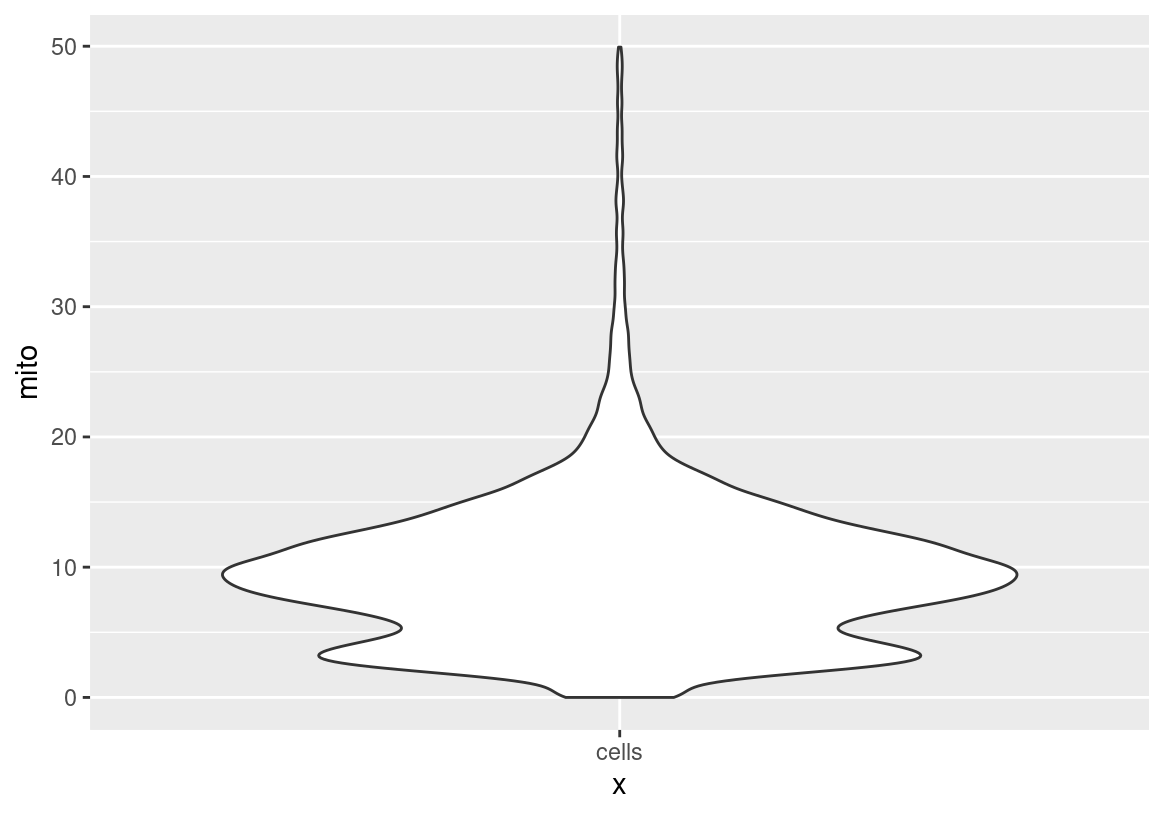
Pre-Process: Remove Doublets
# doublets removal
sc <- doScrubletDetect(sc, return_gobject = TRUE, seed = 0)
ggplot(spatValues(sc, feats = "doublet_scores"), aes(x = "cells", y = doublet_scores)) + geom_violin()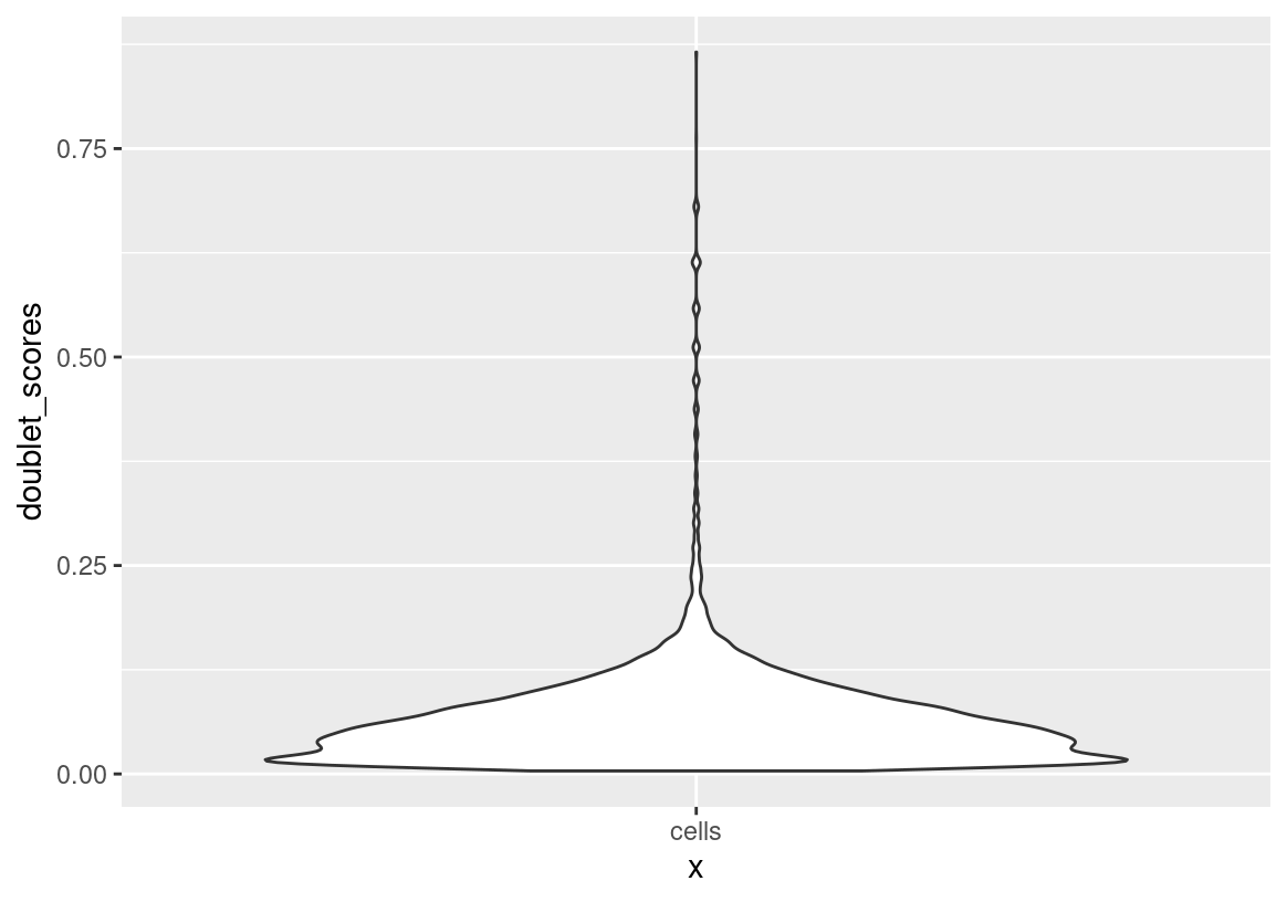
sc <- subset(sc, subset = doublet == FALSE) # remove 130 cellsProcess Data
filterCombinations(sc,
    expression_thresholds = 1,
    feat_det_in_min_cells = c(20, 100)
)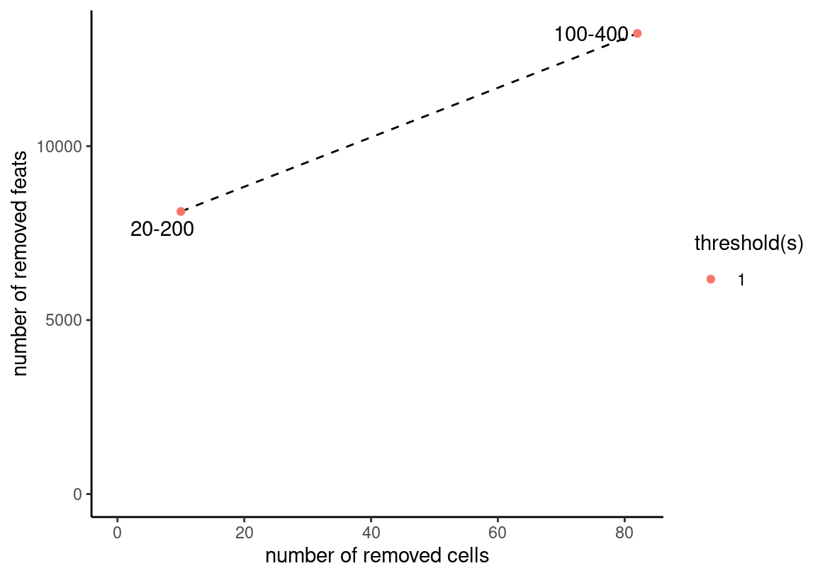
sc <- sc |>
    filterGiotto(
        expression_threshold = 1,
        feat_det_in_min_cells = 20,
        min_det_feats_per_cell = 200
    ) |>
    normalizeGiotto() |>
    calculateHVF() |>
    runPCA()

screePlot(sc, ncp = 50)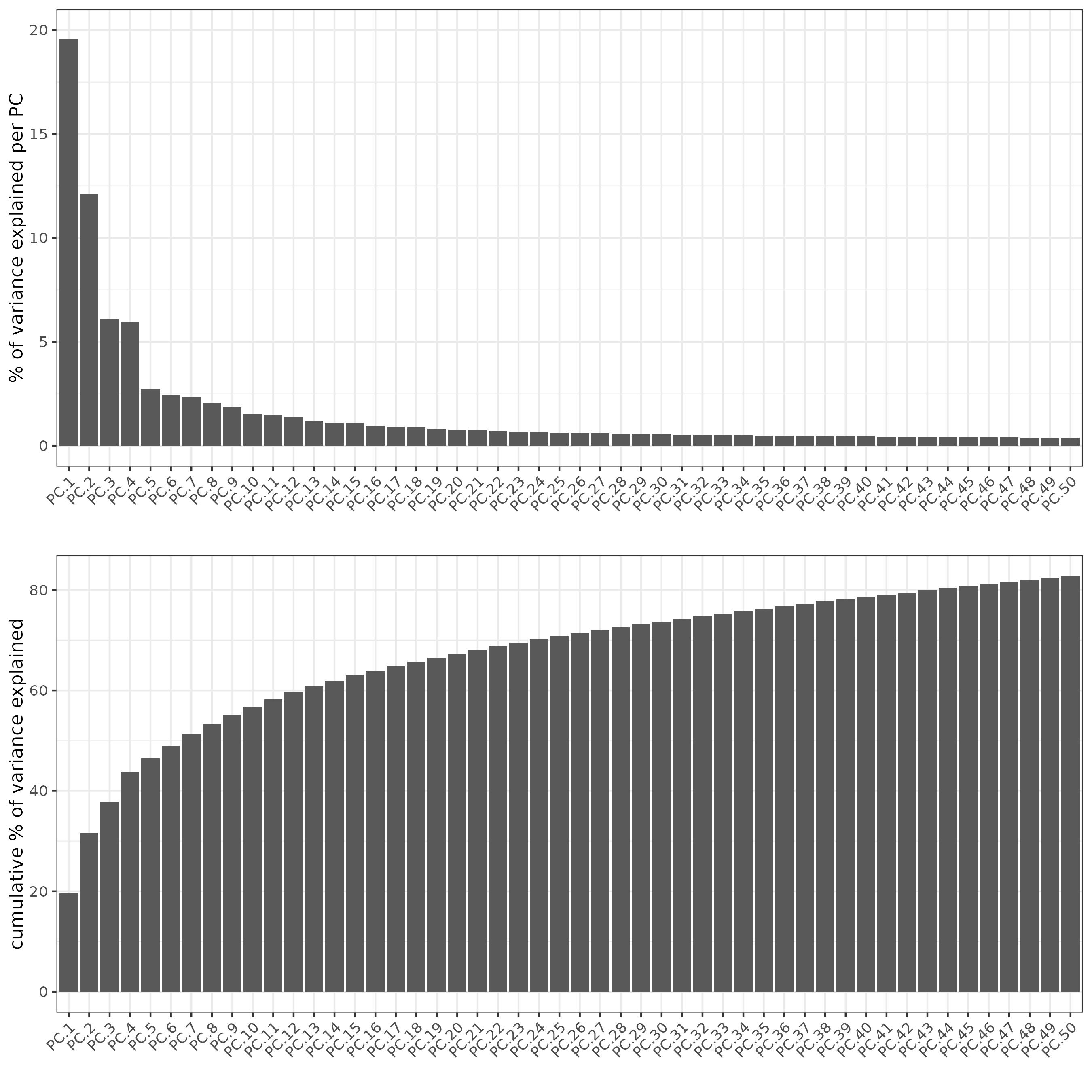
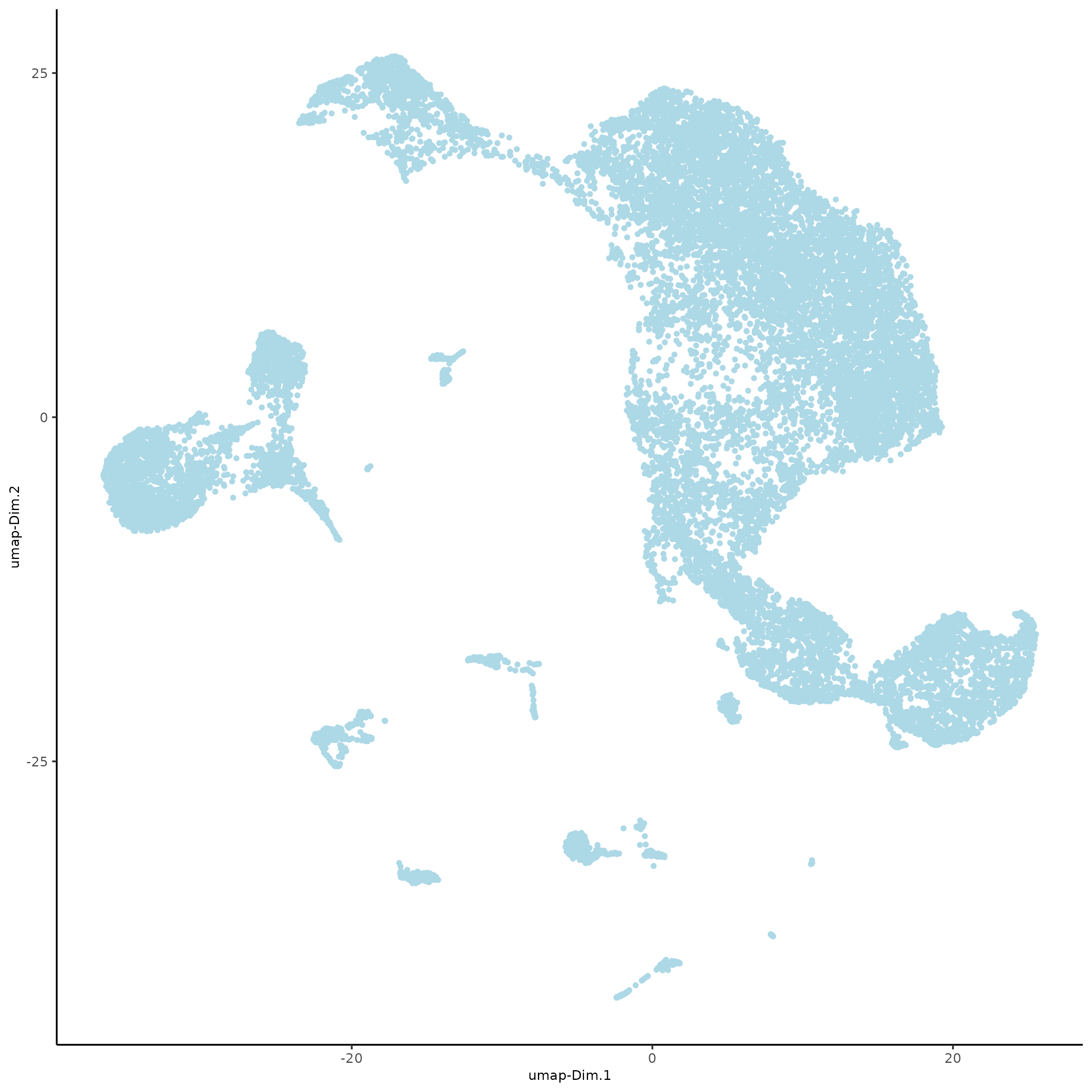
Clustering
sc <- sc |>
    createNearestNetwork(dimensions_to_use = seq(30)) |>
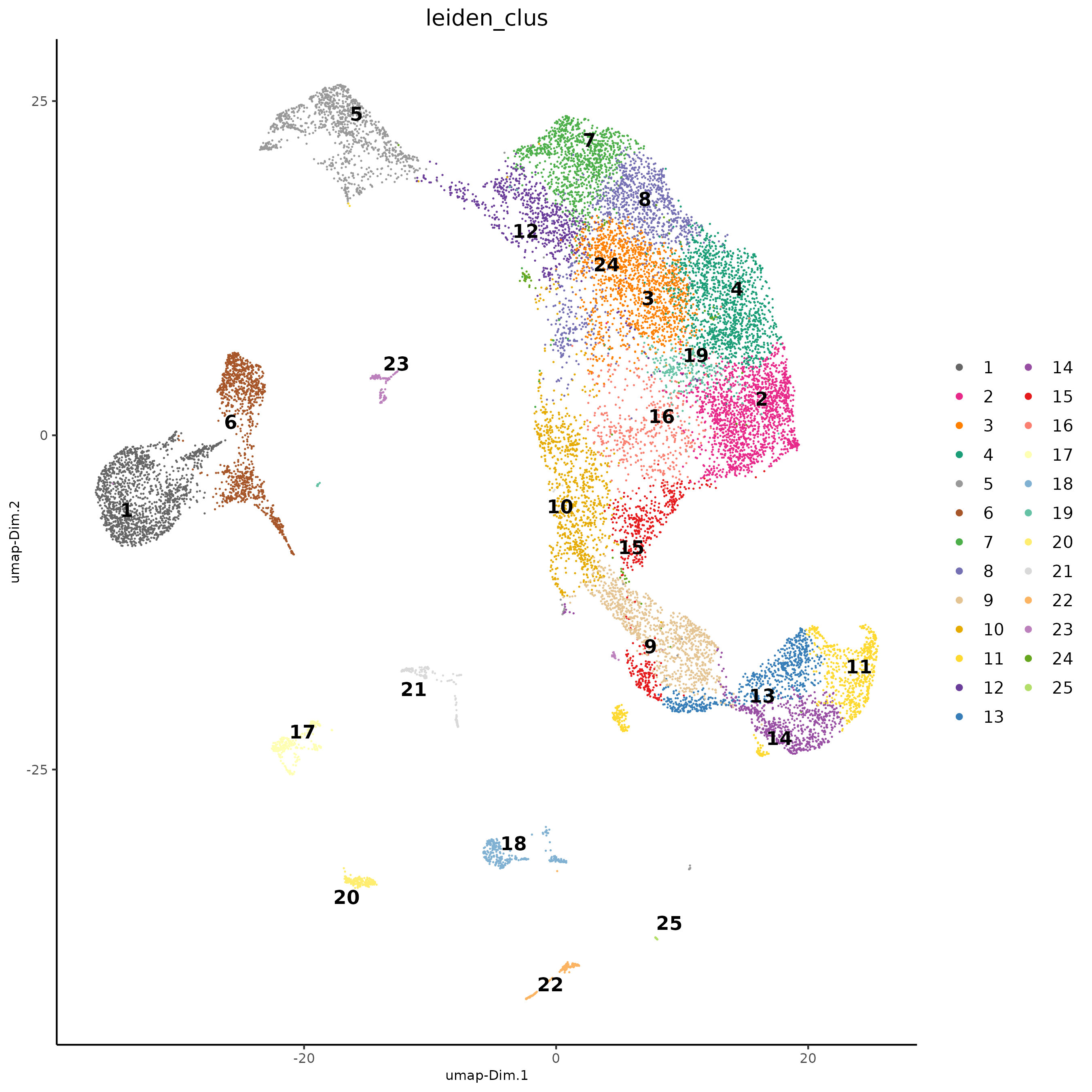
    doLeidenCluster(res = 1.5) # overclustering

dimPlot2D(sc,
    cell_color = "leiden_clus",
    point_size = 0.6,
    point_border_stroke = 0
)
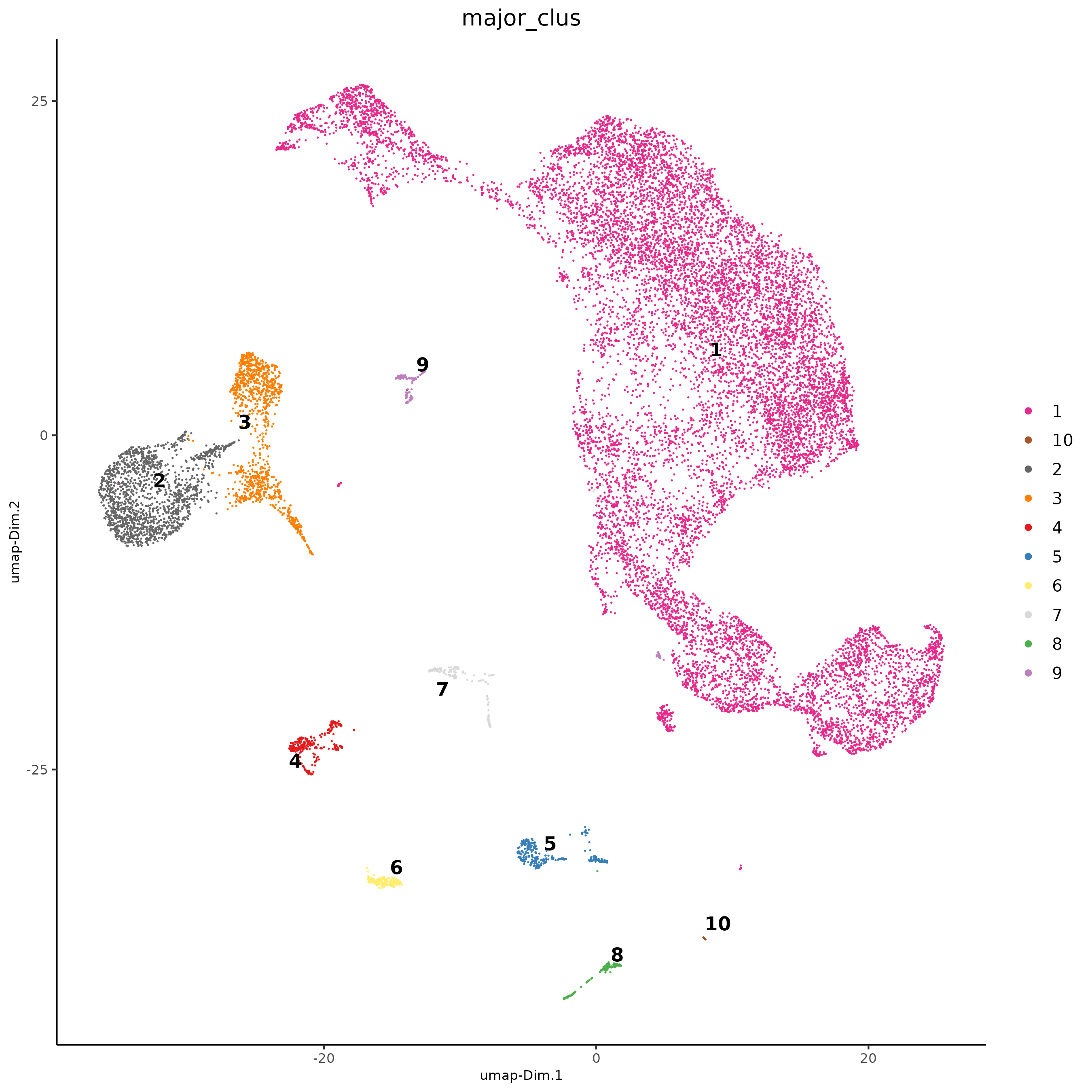
# combine similar clusters
ann <- as.character(seq(25)) |>
    setNames(seq(25))
ann[c(2,3,4,5,7,8,9,10,11,12,13,14,15,16,19,24)] <- 1
ann[c(1,6,17,18,20,21,22,23,25)] <- 2:10

sc <- annotateGiotto(sc,
    annotation_vector = ann,
    cluster_column = "leiden_clus",
    name = "major_clus"
)

dimPlot2D(sc,
    cell_color = "major_clus",
    point_size = 0.6,
    point_border_stroke = 0
)
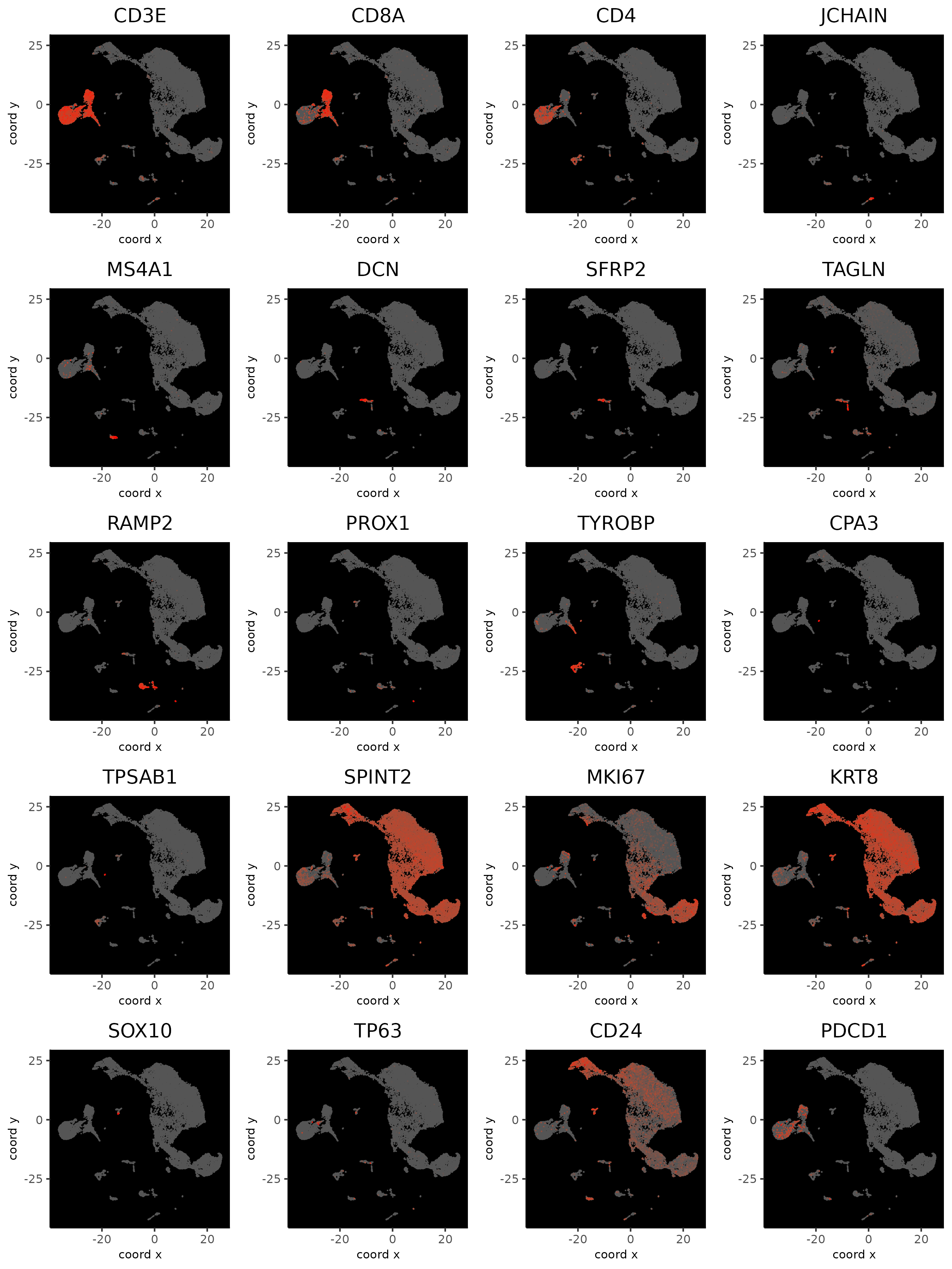
Plot Known Markers
dimFeatPlot2D(sc,
    feats = c(
        "CD3E", "CD8A", "CD4", # T cell
        "JCHAIN", # plasmablast
        "MS4A1", # B
        "DCN", "SFRP2", # CAF (mesenchymal)
        "TAGLN", # CAF/PVL (mesenchymal)
        "RAMP2", # endothelial
        "PROX1", # LEC (lymphatic endothelial cell)
        "TYROBP", # myeloid
        "CPA3", "TPSAB1", # mast cell
        "SPINT2", "MKI67", "KRT8", # epithelial/cancer
        "SOX10", "TP63", # myoepithelial
        "CD24", # B cell and cancer stemness
        "PDCD1" # PD1
    ),
    point_size = 0.5,
    point_border_stroke = 0,
    background_color = "black",
    cow_n_col = 4,
    show_legend = FALSE,
    cell_color_gradient = c("#555555", "red"),
    save_param = list(
      "base_height" = 12
    )
)
Marker Detection: Scran
res_scran <- findMarkers_one_vs_all(sc,
    cluster_column = "major_clus",
    method = "scran"
)
topgenes_scran = res_scran[, head(.SD, 2), by = 'cluster']
violinPlot(sc, feats = topgenes_scran$feats, cluster_column = "major_clus")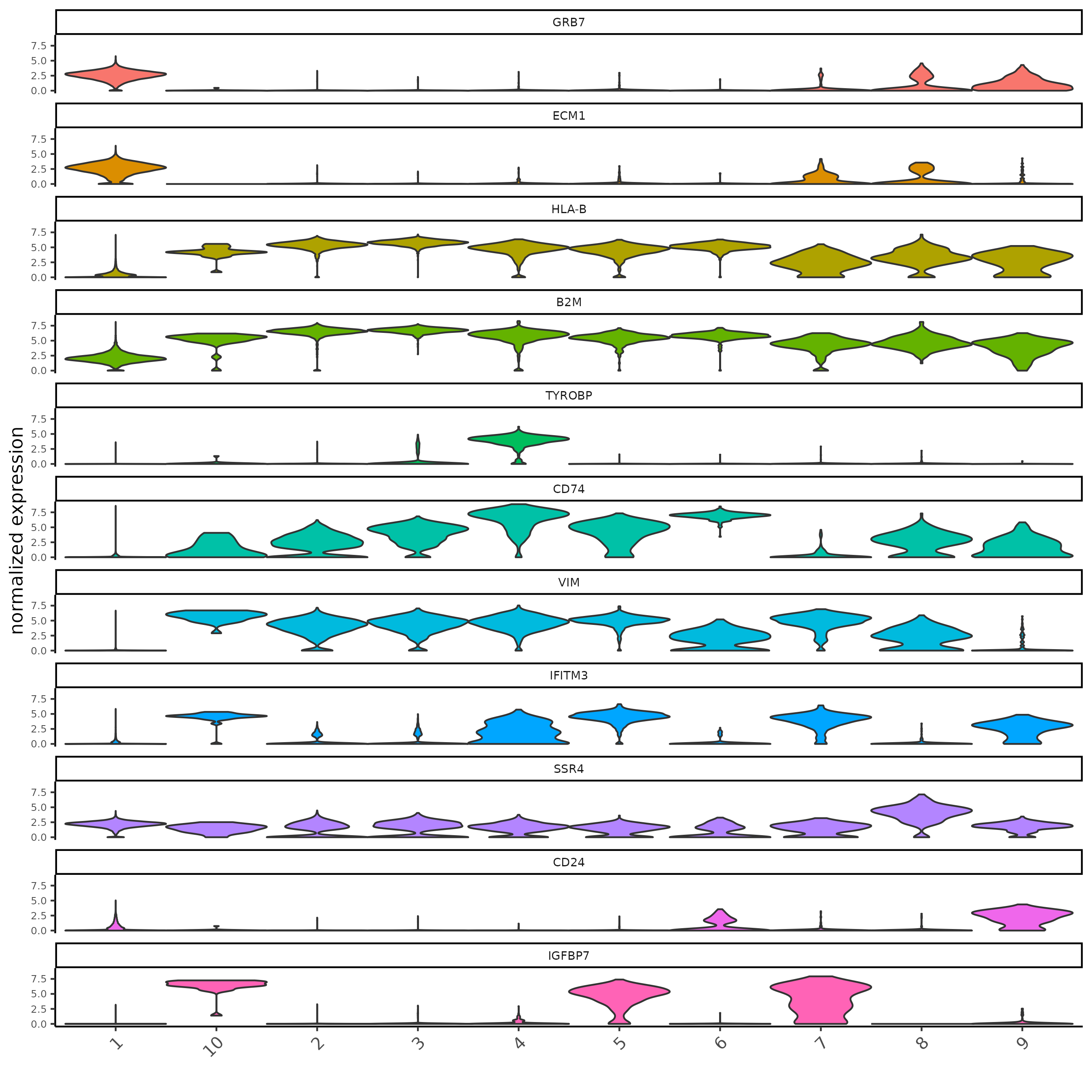
Marker Detection: Gini
res_gini <- findMarkers_one_vs_all(sc,
    cluster_column = "major_clus",
    method = "gini"
)
topgenes_gini = res_gini[, head(.SD, 2), by = 'cluster']
violinPlot(sc, feats = topgenes_gini$feats, cluster_column = "major_clus")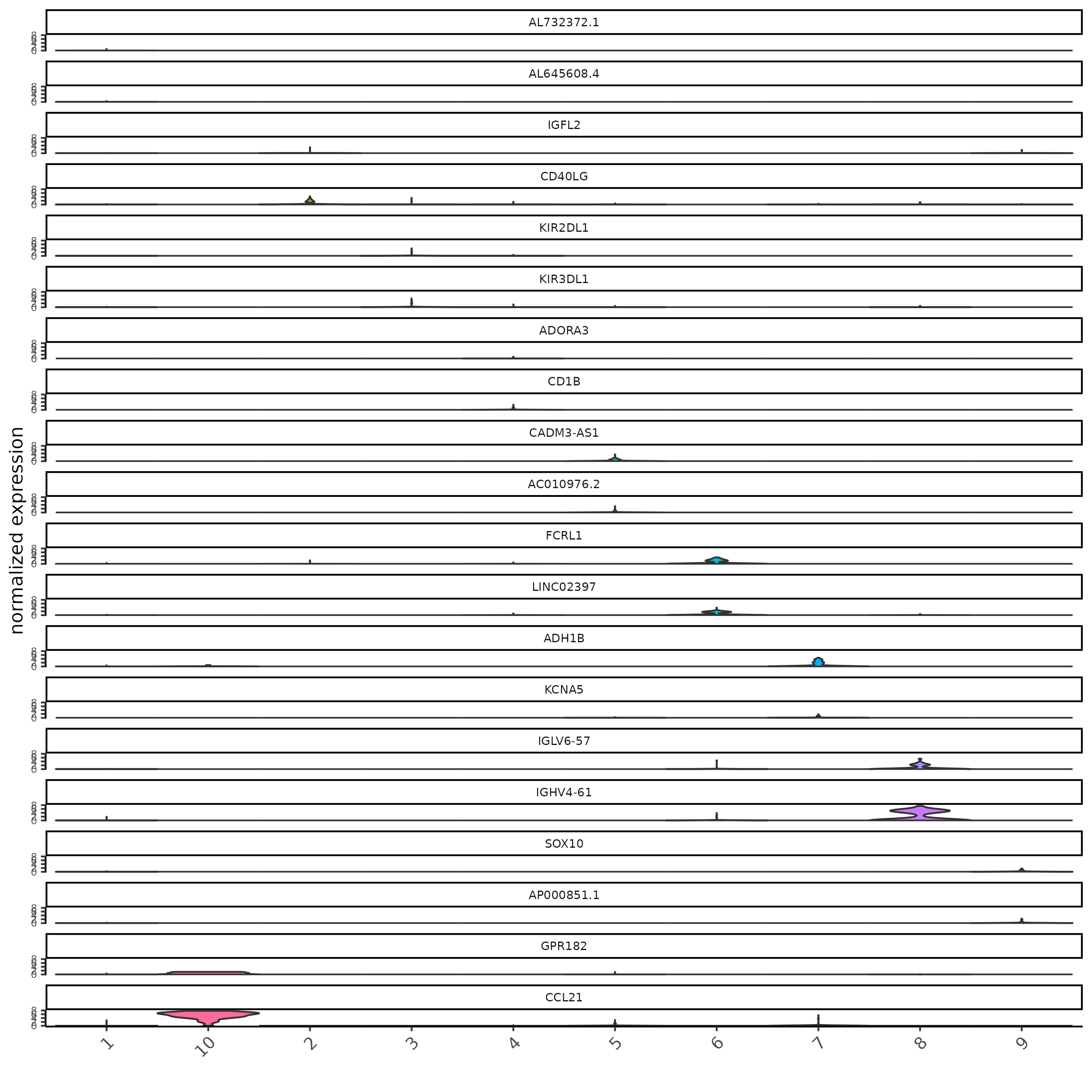
Annotate: Major Cell Types
ann2 <- c(
    "cancer_epithelial",
    "CD4T",
    "CD8T",
    "myeloid",
    "endothelial",
    "B",
    "mesenchymal",
    "plasmablast",
    "myoepithelial",
    "LEC"
) |>
    setNames(seq(10))

sc <- annotateGiotto(sc,
    cluster_column = "major_clus",
    annotation_vector = ann2,
    name = "cell_types"
)

dimPlot2D(sc, cell_color = "cell_types")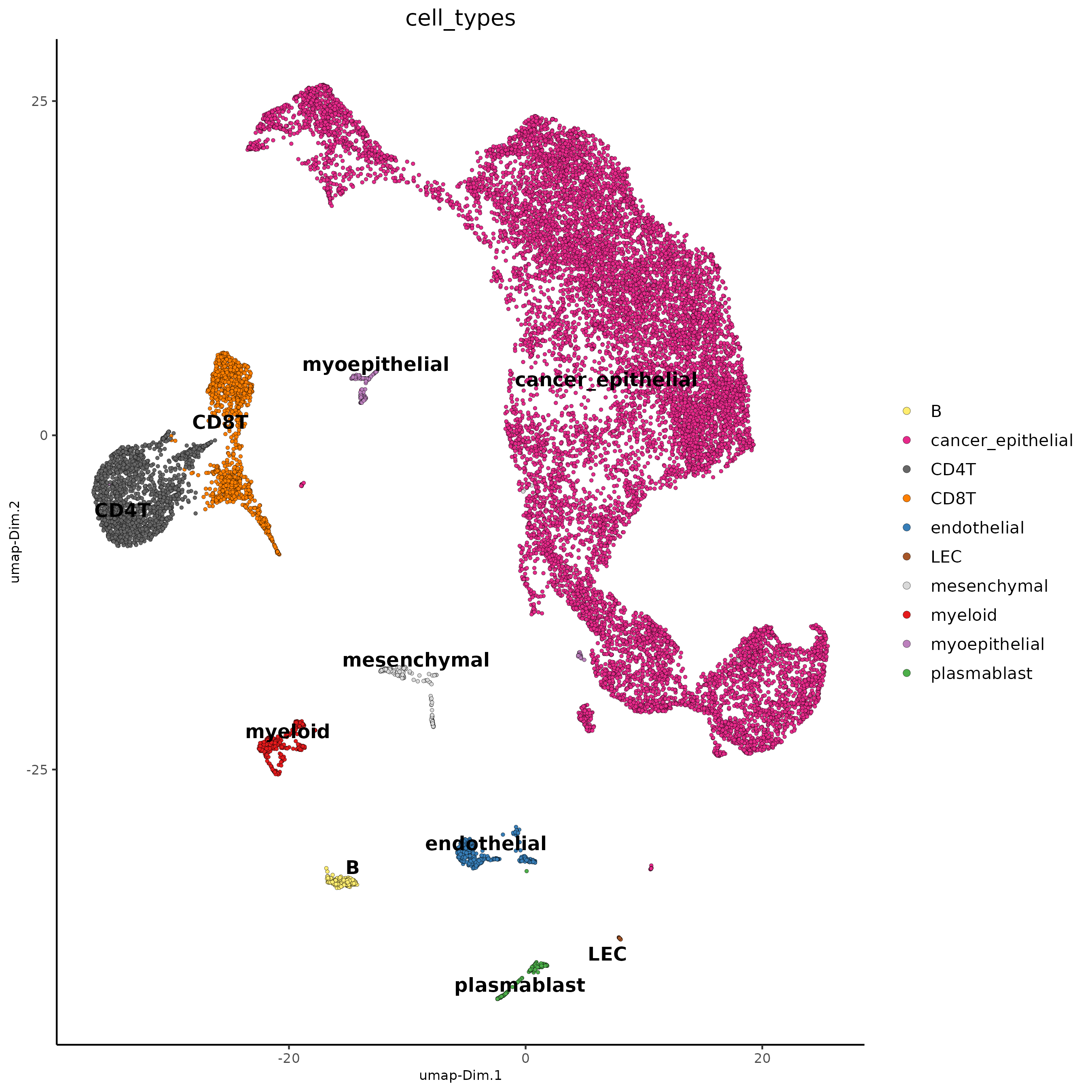
6.2 Create Joined Object
Next, a joined Xenium and single cell giotto object
needs to be created to transfer the cell type labels.
# match features
ufids <- intersect(featIDs(xenium_gobj), featIDs(sc)) # 298 feats in common

# strip gobjects down to remove incompatible elements in join
sc_join <- giotto() |>
    setGiotto(sc[[c("expression", "spatial_locs"), "raw"]])
xen_join <- giotto() |>
    setGiotto(xenium_gobj[[c("expression", "spatial_locs"), "raw", spat_unit = "cell"]])

j <- joinGiottoObjects(
    list(sc_join[ufids], xen_join[ufids]),
    gobject_names = c("sc", "xen")
)
instructions(j) <- instrs
6.3 Process Joined Object (No Integration)
j <- filterGiotto(j,
    expression_threshold = 1,
    feat_det_in_min_cells = 1,
    min_det_feats_per_cell = 10
)
# normalizations
j <- normalizeGiotto(j) # pearson and quantile norms do not work well for this

# PCA
j <- runPCA(j, feats_to_use = NULL)

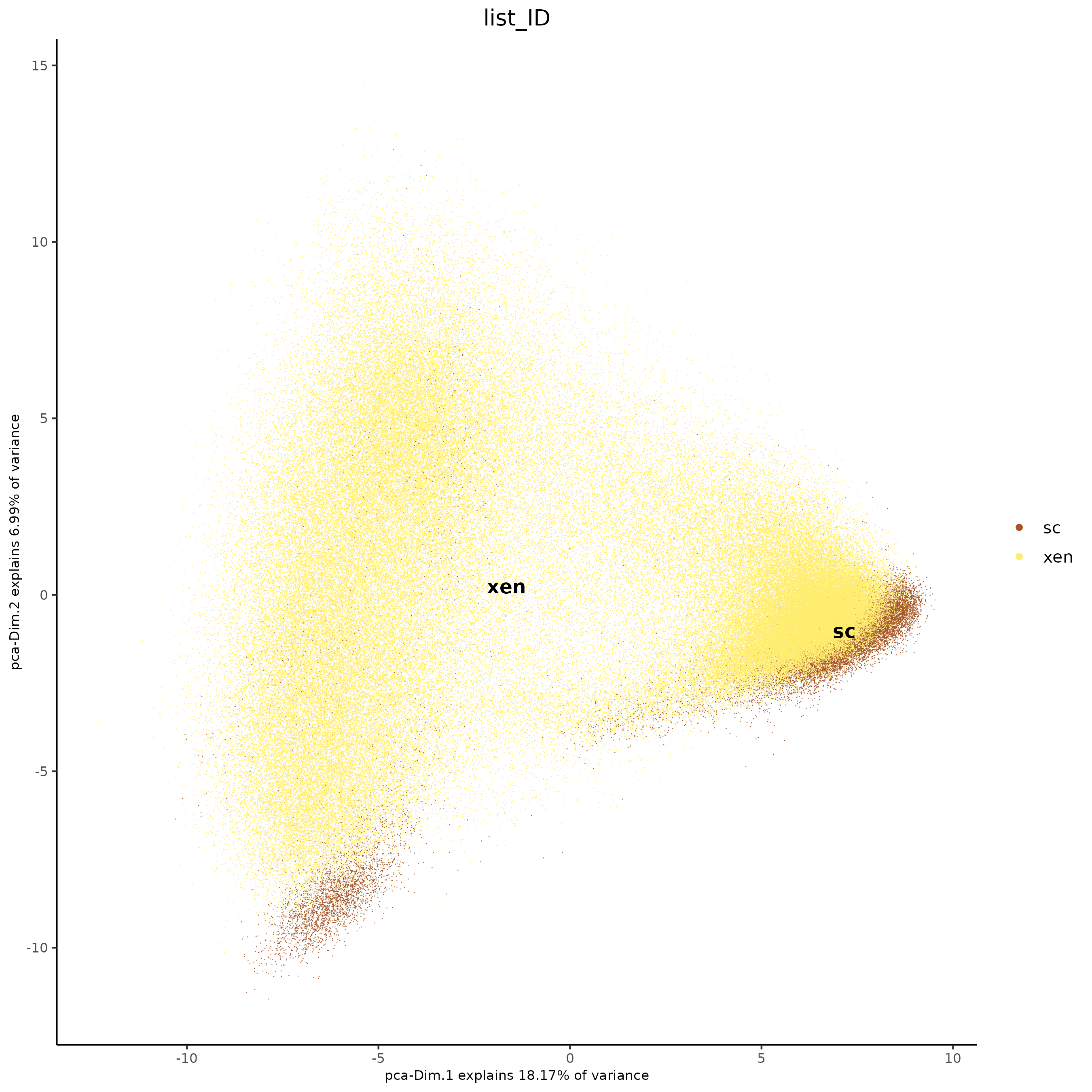
plotPCA(j,
    cell_color = "list_ID",
    point_border_stroke = 0,
    point_size = 0.3
)
screePlot(j, ncp = 50)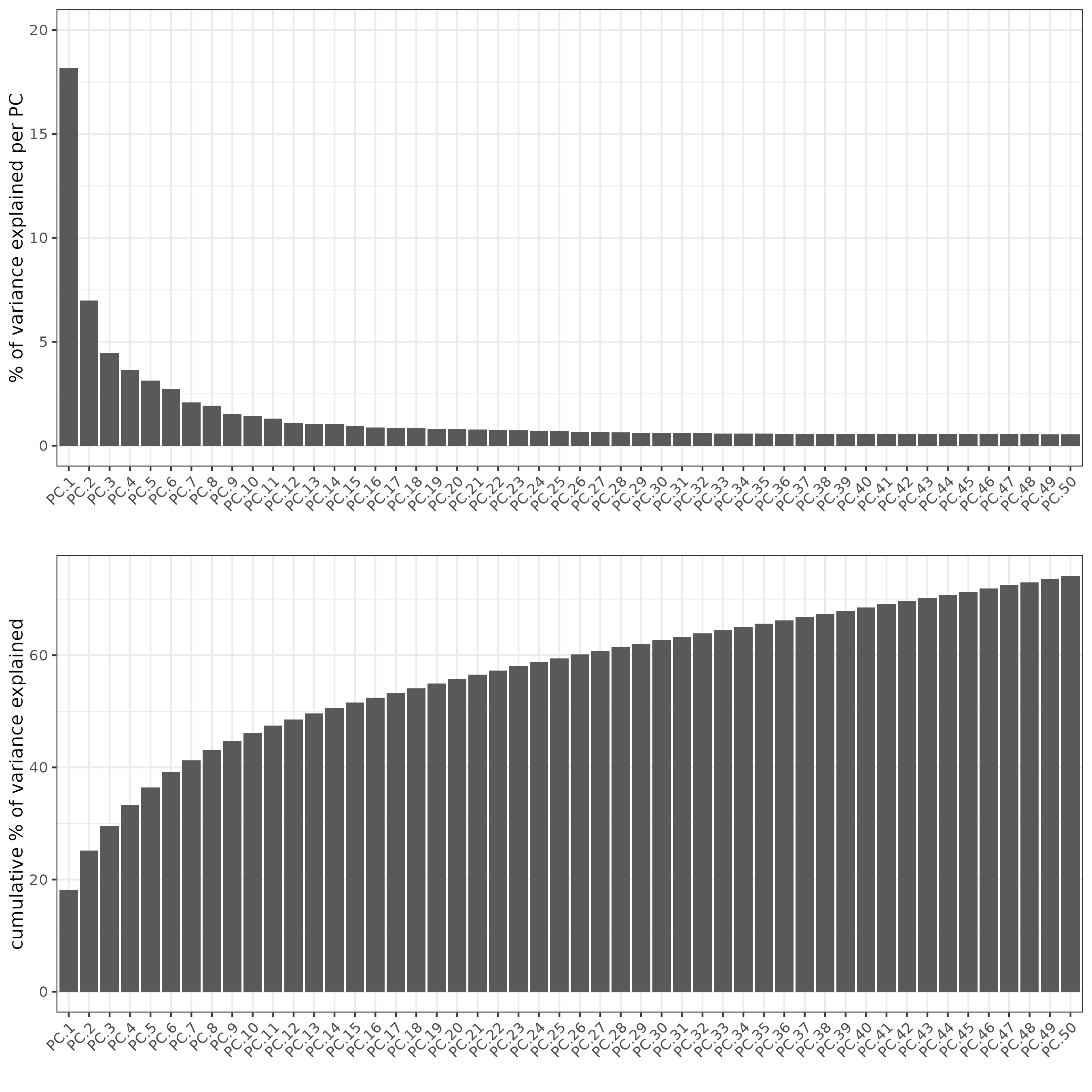
ndims <- 10
j <- runUMAP(j, dimensions_to_use = seq(ndims))

plotUMAP(j,
    cell_color = "list_ID",
    point_size = 0.3,
    point_border_stroke = 0,
    cell_color_code = c("red", "blue")
)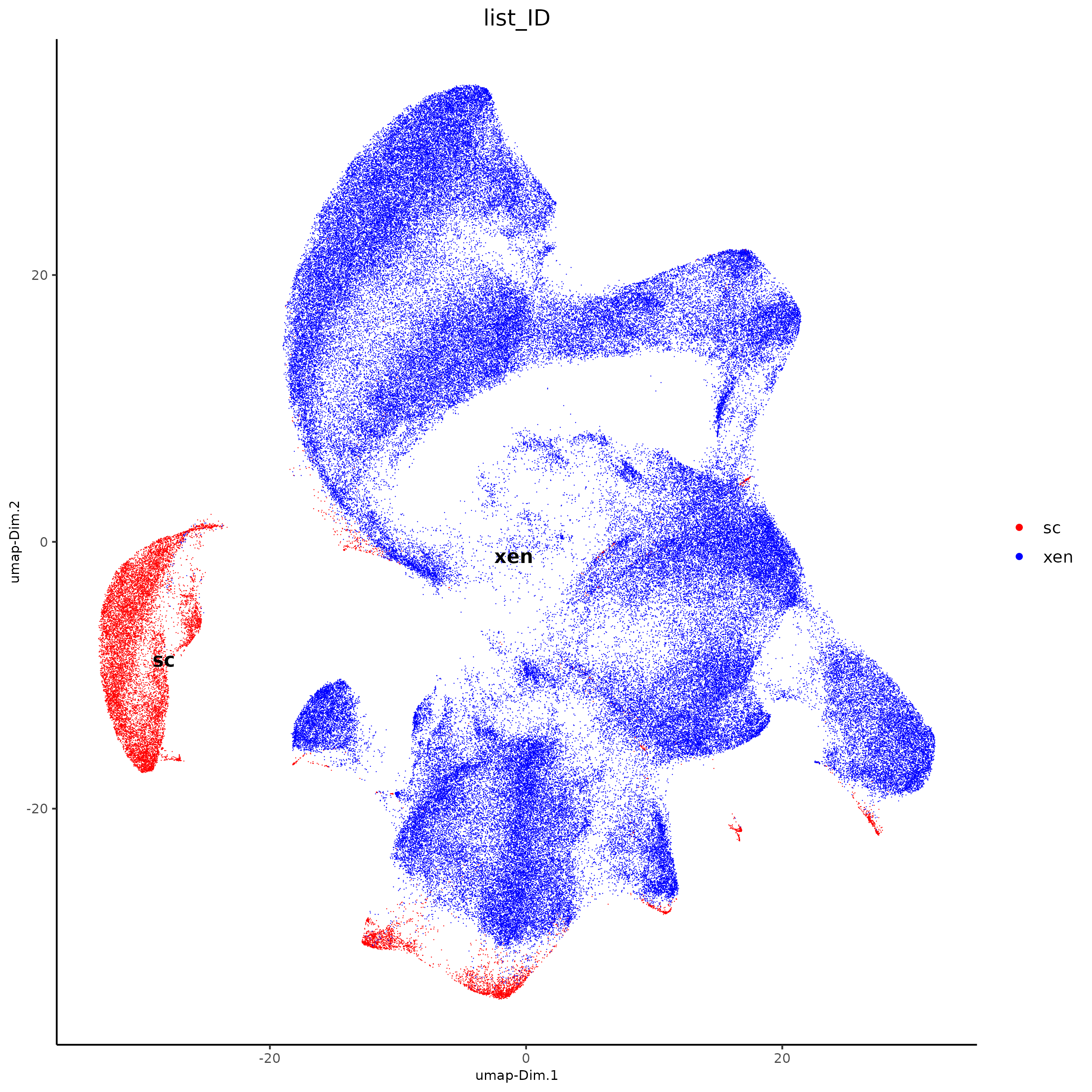
There are clear batch effects between the two types of data, so we can try Harmony integration.
6.4 Process Joined Object (With Harmony Integration)
Run Harmony integration on the PCA space with the
"list_ID" (dataset source) as the variable to remove to
produce an aligned PCA space that better represents the biology of the
datasets.
j <- runGiottoHarmony(j,
    vars_use = "list_ID",
    dim_reduction_name = "pca",
    dimensions_to_use = seq(ndims),
    name = "harmony"
)

j <- runUMAP(j,
    dim_reduction_to_use = "harmony",
    dim_reduction_name = "harmony",
    name = "umap_harmony",
    dimensions_to_use = seq(ndims)
)

cell_colors <- c(
    "turquoise", "azure4", "pink", "tomato",
    "chartreuse3", "lightslateblue", "firebrick4",
    "blue", "magenta", "cornflowerblue"
)

plotUMAP(j,
    cell_color = "cell_types",
    dim_reduction_name = "umap_harmony",
    cell_color_code = cell_colors,
    point_size = 0.5,
    select_cells = spatIDs(j, subset = list_ID == "sc"),
    point_border_stroke = 0,
    other_point_size = 0.3
)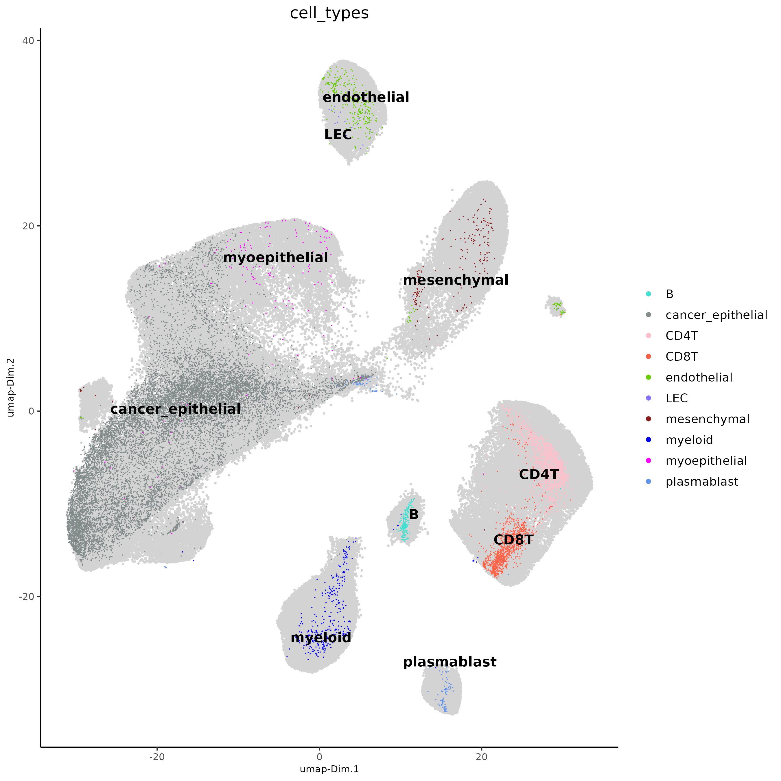
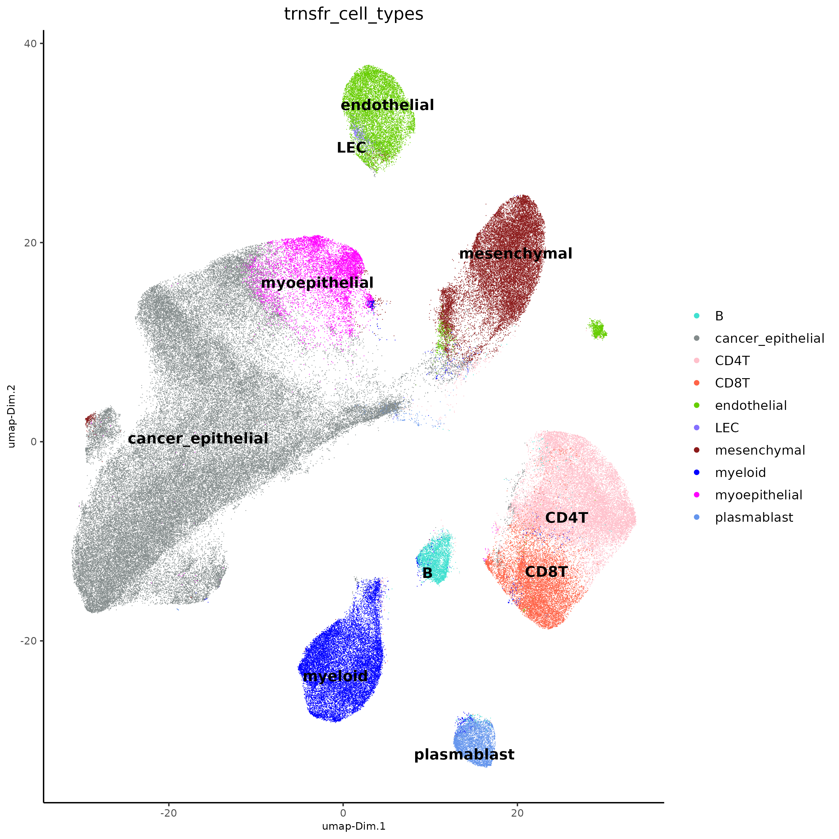
The single-cell-based celltype annotations look like they map to the
clustering of the integrated dataset. We can now transfer these
annotations using labelTransfer() from just the single
cells (source_cell_ids) to the rest of the cells (xenium
data cells) using kNN clustering.
j <- labelTransfer(j,
    source_cell_ids = spatIDs(j, subset = list_ID == "sc"),
    k = 10,
    labels = "cell_types",
    reduction_method = "harmony",
    reduction_name = "harmony",
    dimensions_to_use = seq(ndims)
)

plotUMAP(j,
    cell_color = "trnsfr_cell_types",
    dim_reduction_name = "umap_harmony",
    cell_color_code = cell_colors,
    point_size = 0.3,
    point_border_stroke = 0
)
ann_meta <- pDataDT(j)
ann_meta <- ann_meta[list_ID == "xen",]
ann_meta[, cell_ID := gsub("^xen-", "", cell_ID)]
ann_meta <- ann_meta[, .(cell_ID, trnsfr_cell_types, trnsfr_cell_types_prob)]

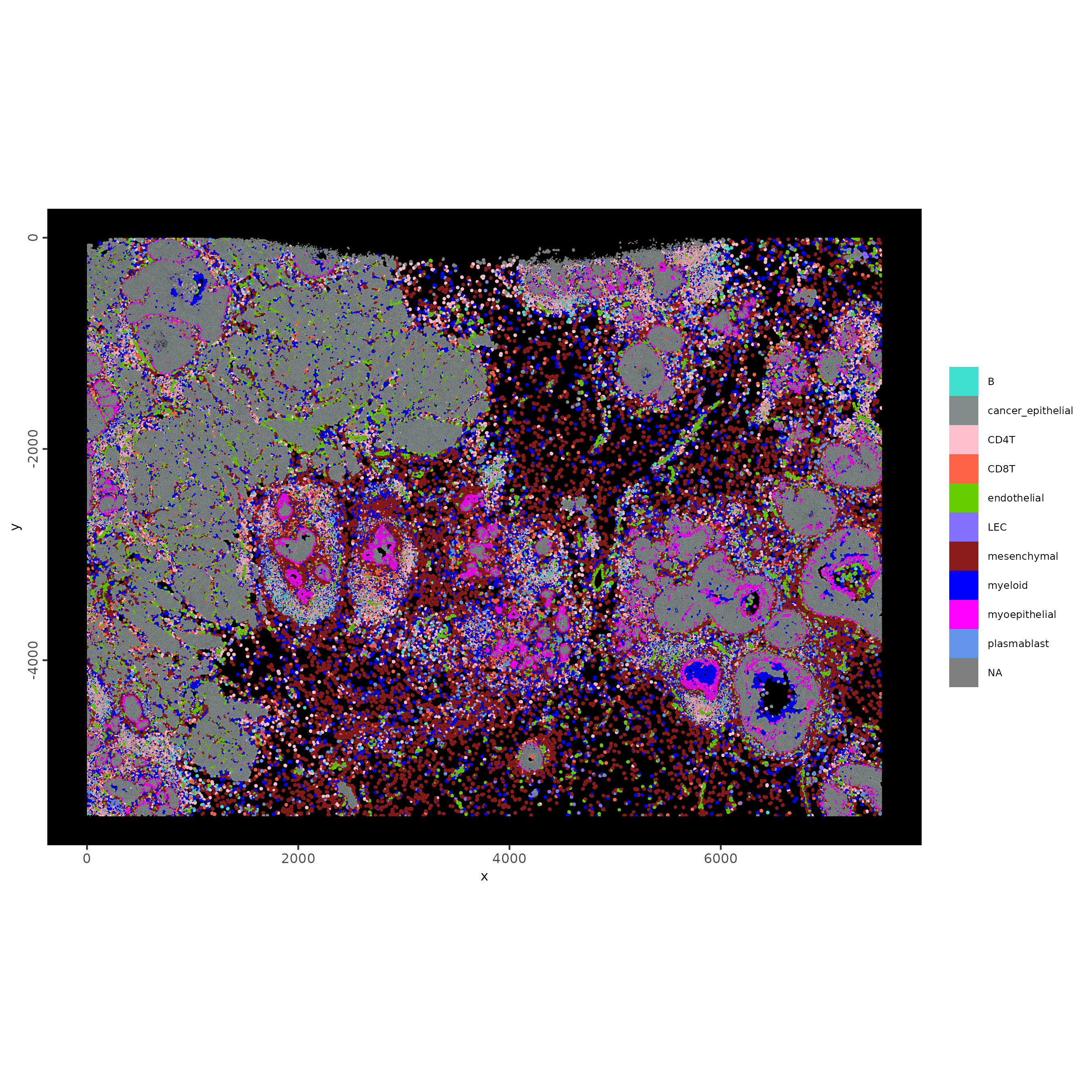
xenium_gobj <- addCellMetadata(xenium_gobj,
    new_metadata = ann_meta,
    by_column = TRUE,
    column_cell_ID = "cell_ID"
)

spatInSituPlotPoints(xenium_gobj,
    polygon_fill = "trnsfr_cell_types",
    polygon_fill_as_factor = TRUE,
    polygon_line_size = 0,
    polygon_fill_code = cell_colors
)
res <- labelTransfer(xenium_gobj, sc,
    labels = "cell_types",
    integration_method = "harmony",
    k = 10,
    dimensions_to_use = seq(ndims)
)R version 4.4.0 (2024-04-24)
Platform: x86_64-pc-linux-gnu
Running under: AlmaLinux 8.10 (Cerulean Leopard)
Matrix products: default
BLAS/LAPACK: FlexiBLAS NETLIB; LAPACK version 3.11.0
locale:
[1] LC_CTYPE=en_US.UTF-8 LC_NUMERIC=C LC_TIME=en_US.UTF-8
[4] LC_COLLATE=en_US.UTF-8 LC_MONETARY=en_US.UTF-8 LC_MESSAGES=en_US.UTF-8
[7] LC_PAPER=en_US.UTF-8 LC_NAME=C LC_ADDRESS=C
[10] LC_TELEPHONE=C LC_MEASUREMENT=en_US.UTF-8 LC_IDENTIFICATION=C
time zone: America/New_York
tzcode source: system (glibc)
attached base packages:
[1] stats graphics grDevices utils datasets methods base
other attached packages:
[1] ggplot2_3.5.1 Giotto_4.1.5 GiottoClass_0.4.4
loaded via a namespace (and not attached):
[1] RColorBrewer_1.1-3 rstudioapi_0.16.0 jsonlite_1.8.8
[4] magrittr_2.0.3 magick_2.8.4 farver_2.1.2
[7] rmarkdown_2.28 zlibbioc_1.50.0 ragg_1.3.0
[10] vctrs_0.6.5 DelayedMatrixStats_1.26.0 GiottoUtils_0.2.1
[13] terra_1.7-78 htmltools_0.5.8.1 S4Arrays_1.4.1
[16] BiocNeighbors_1.22.0 tictoc_1.2.1 Rhdf5lib_1.26.0
[19] SparseArray_1.4.8 rhdf5_2.48.0 parallelly_1.37.1
[22] htmlwidgets_1.6.4 plotly_4.10.4 igraph_2.0.3
[25] lifecycle_1.0.4 pkgconfig_2.0.3 rsvd_1.0.5
[28] Matrix_1.7-0 R6_2.5.1 fastmap_1.2.0
[31] GenomeInfoDbData_1.2.12 MatrixGenerics_1.16.0 future_1.33.2
[34] digest_0.6.37 colorspace_2.1-1 S4Vectors_0.42.1
[37] dqrng_0.4.1 irlba_2.3.5.1 textshaping_0.3.7
[40] GenomicRanges_1.56.0 beachmat_2.20.0 labeling_0.4.3
[43] progressr_0.14.0 fansi_1.0.6 httr_1.4.7
[46] abind_1.4-5 compiler_4.4.0 bit64_4.0.5
[49] withr_3.0.1 backports_1.5.0 BiocParallel_1.38.0
[52] DBI_1.2.3 qs_0.26.3 pak_0.7.2
[55] R.utils_2.12.3 duckdb_1.0.0-2 rappdirs_0.3.3
[58] DelayedArray_0.30.1 bluster_1.14.0 rjson_0.2.21
[61] gtools_3.9.5 GiottoVisuals_0.2.9 tools_4.4.0
[64] future.apply_1.11.2 R.oo_1.26.0 glue_1.7.0
[67] dbscan_1.2-0 rhdf5filters_1.16.0 grid_4.4.0
[70] job_0.3.1 checkmate_2.3.2 cluster_2.1.6
[73] generics_0.1.3 hdf5r_1.3.11 gtable_0.3.5
[76] R.methodsS3_1.8.2 tidyr_1.3.1 data.table_1.16.0
[79] RApiSerialize_0.1.3 metapod_1.12.0 BiocSingular_1.20.0
[82] ScaledMatrix_1.12.0 stringfish_0.16.0 utf8_1.2.4
[85] XVector_0.44.0 BiocGenerics_0.50.0 RcppAnnoy_0.0.22
[88] ggrepel_0.9.6 pillar_1.9.0 limma_3.60.2
[91] later_1.3.2 dplyr_1.1.4 lattice_0.22-6
[94] FNN_1.1.4 bit_4.0.5 pool_1.0.3
[97] tidyselect_1.2.1 locfit_1.5-9.10 SingleCellExperiment_1.26.0
[100] scuttle_1.14.0 knitr_1.48 IRanges_2.38.0
[103] edgeR_4.2.0 SummarizedExperiment_1.34.0 scattermore_1.2
[106] RhpcBLASctl_0.23-42 stats4_4.4.0 xfun_0.47
[109] Biobase_2.64.0 statmod_1.5.0 matrixStats_1.4.1
[112] UCSC.utils_1.0.0 lazyeval_0.2.2 yaml_2.3.10
[115] evaluate_0.24.0 codetools_0.2-20 GiottoData_0.2.14
[118] tibble_3.2.1 colorRamp2_0.1.0 cli_3.6.3
[121] uwot_0.2.2 RcppParallel_5.1.7 arrow_16.1.0
[124] reticulate_1.38.0 systemfonts_1.1.0 munsell_0.5.1
[127] harmony_1.2.0 Rcpp_1.0.13 GenomeInfoDb_1.40.0
[130] globals_0.16.3 png_0.1-8 parallel_4.4.0
[133] assertthat_0.2.1 scran_1.32.0 sparseMatrixStats_1.16.0
[136] listenv_0.9.1 SpatialExperiment_1.14.0 viridisLite_0.4.2
[139] scales_1.3.0 purrr_1.0.2 crayon_1.5.2
[142] rlang_1.1.4 cowplot_1.1.3