1 Ensure Giotto and GiottoData are installed
# Ensure Giotto Suite is installed.
if(!"Giotto" %in% installed.packages()) {
  pak::pkg_install("drieslab/Giotto")
}
# Ensure the Python environment for Giotto has been installed.
genv_exists <- Giotto::checkGiottoEnvironment()
if(!genv_exists){
  # The following command need only be run once to install the Giotto environment.
  Giotto::installGiottoEnvironment()
}

# Ensure GiottoData is installed.
if(!"GiottoData" %in% installed.packages()) {
  pak::pkg_install("drieslab/GiottoData")
}

library(Giotto)
Aggregate datasets are ones where the features information has already been aggregated and you are starting with an expression matrix and a set of xy(z) coordinates.
This example will be shown using an osmFISH dataset. To download this data, please ensure that wget is installed locally.
2 Download data to use
# Specify path from which data may be retrieved/stored
data_path <- "/path/to/data/"

# Download osmFISH dataset to data_path
GiottoData::getSpatialDataset(
    dataset = "osmfish_SS_cortex",
    directory = data_path,
    method = "wget"
)
3 Read data into Giotto Suite
Aggregate data (matrix and spatial locations -based data) can be read
in using createGiottoObject(). There are two examples. Data
formatting guidelines are shown below this code block.
# Example 1.
# Create a giotto object using data directly from file paths
osm_exprs <- file.path(data_path, "osmFISH_prep_expression.txt")
osm_locs <- file.path(data_path, "osmFISH_prep_cell_coordinates.txt")

minimum_gobject1 <- createGiottoObject(
    expression = osm_exprs,
    spatial_locs = osm_locs
)
force(minimum_gobject1)
An object of class giotto
>Active spat_unit: cell
>Active feat_type: rna
dimensions : 33, 5328 (features, cells)
[SUBCELLULAR INFO]
[AGGREGATE INFO]
expression -----------------------
[cell][rna] raw
spatial locations ----------------
[cell] raw
Use objHistory() to see steps and params used
# Example 2.
# Create a giotto object using objects already loaded into workspace
# readExprMatrix will load matrix formats into memory as a Matrix format
expression_matrix <- readExprMatrix(path = osm_exprs) # fast method to read expression matrix
cell_locations <- data.table::fread(file = osm_locs)

minimum_gobject2 <- createGiottoObject(
    expression = expression_matrix,
    spatial_locs = cell_locations
)
force(minimum_gobject2)
An object of class giotto
>Active spat_unit: cell
>Active feat_type: rna
dimensions : 33, 5328 (features, cells)
[SUBCELLULAR INFO]
[AGGREGATE INFO]
expression -----------------------
[cell][rna] raw
spatial locations ----------------
[cell] raw
Use objHistory() to see steps and params used4 Example plot
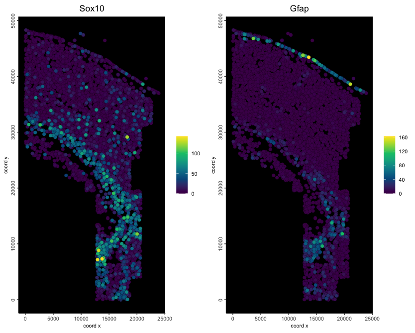
spatFeatPlot2D(minimum_gobject1,
    feats = c("Sox10", "Gfap"),
    expression_values = "raw",
    point_size = 2.5,
    gradient_style = "sequential",
    background_color = "black"
)
5 Data formatting notes
Expression file formatting
Expression count matrices accepted by Giotto should be oriented with columns corresponding to individual cells/observations (cell IDs) and rows to individual features (feature IDs). It is also preferred for the rows and cols to be named by the features and cells they describe.
matrix and DelayedMatrix objects should have the feature IDs already incorporated as the rownames.
data.table objects and text-based files ie: (.csv, .tsv, .txt) to be read in should have column 1 be feature IDs.
Locations file formatting
- Numerical columns will be interpreted in order of x, y, and (optionally) z coordinate. The first non-numerical column will be taken as cell IDs
*Note:
multiple expression files during can be given at once during Giotto object creation by using a named list.
# Example where additional matrices are added during object creation

# Arbitrary modifications
scaled_matrix <- expression_matrix * 1.2
custom_matrix <- expression_matrix * 0.5

# Provide multiple expression matrices at once to the Giotto Object
# If these matrices are stored in files rather than in the workspace,
# file paths may be provided instead of variables
multi_expr_gobject <- createGiottoObject(
    expression = list( # named list of multiple expression matrices
        raw = expression_matrix,
        scaled = scaled_matrix,
        custom = custom_matrix
    ),
    spatial_locs = cell_locations
)
force(multi_expr_gobject)
An object of class giotto
>Active spat_unit: cell
>Active feat_type: rna
dimensions : 33, 5328 (features, cells)
[SUBCELLULAR INFO]
[AGGREGATE INFO]
expression -----------------------
[cell][rna] raw scaled custom
spatial locations ----------------
[cell] raw
Use objHistory() to see steps and params used6 Session Info
R version 4.4.1 (2024-06-14)
Platform: aarch64-apple-darwin20
Running under: macOS 15.0.1

Matrix products: default
BLAS:   /System/Library/Frameworks/Accelerate.framework/Versions/A/Frameworks/vecLib.framework/Versions/A/libBLAS.dylib
LAPACK: /Library/Frameworks/R.framework/Versions/4.4-arm64/Resources/lib/libRlapack.dylib;  LAPACK version 3.12.0

locale:
[1] en_US.UTF-8/en_US.UTF-8/en_US.UTF-8/C/en_US.UTF-8/en_US.UTF-8

time zone: America/New_York
tzcode source: internal

attached base packages:
[1] stats     graphics  grDevices utils     datasets  methods   base

other attached packages:
[1] Giotto_4.1.5      GiottoClass_0.4.3

loaded via a namespace (and not attached):
 [1] tidyselect_1.2.1            viridisLite_0.4.2           dplyr_1.1.4
 [4] farver_2.1.2                GiottoVisuals_0.2.7         fastmap_1.2.0
 [7] SingleCellExperiment_1.26.0 lazyeval_0.2.2              digest_0.6.37
[10] lifecycle_1.0.4             terra_1.7-78                magrittr_2.0.3
[13] compiler_4.4.1              rlang_1.1.4                 tools_4.4.1
[16] igraph_2.1.1                utf8_1.2.4                  yaml_2.3.10
[19] data.table_1.16.2           knitr_1.48                  labeling_0.4.3
[22] S4Arrays_1.4.0              htmlwidgets_1.6.4           reticulate_1.39.0
[25] DelayedArray_0.30.0         abind_1.4-8                 withr_3.0.1
[28] purrr_1.0.2                 BiocGenerics_0.50.0         grid_4.4.1
[31] stats4_4.4.1                fansi_1.0.6                 colorspace_2.1-1
[34] ggplot2_3.5.1               scales_1.3.0                gtools_3.9.5
[37] SummarizedExperiment_1.34.0 cli_3.6.3                   rmarkdown_2.28
[40] crayon_1.5.3                generics_0.1.3              rstudioapi_0.16.0
[43] httr_1.4.7                  rjson_0.2.21                zlibbioc_1.50.0
[46] parallel_4.4.1              XVector_0.44.0              matrixStats_1.4.1
[49] vctrs_0.6.5                 Matrix_1.7-0                jsonlite_1.8.9
[52] GiottoData_0.2.15           IRanges_2.38.0              S4Vectors_0.42.0
[55] ggrepel_0.9.6               scattermore_1.2             magick_2.8.5
[58] GiottoUtils_0.2.1           plotly_4.10.4               tidyr_1.3.1
[61] glue_1.8.0                  codetools_0.2-20            cowplot_1.1.3
[64] gtable_0.3.5                GenomeInfoDb_1.40.0         GenomicRanges_1.56.0
[67] UCSC.utils_1.0.0            munsell_0.5.1               tibble_3.2.1
[70] pillar_1.9.0                htmltools_0.5.8.1           GenomeInfoDbData_1.2.12
[73] R6_2.5.1                    evaluate_1.0.0              lattice_0.22-6
[76] Biobase_2.64.0              png_0.1-8                   backports_1.5.0
[79] SpatialExperiment_1.14.0    Rcpp_1.0.13                 SparseArray_1.4.1
[82] checkmate_2.3.2             colorRamp2_0.1.0            xfun_0.47
[85] MatrixGenerics_1.16.0       pkgconfig_2.0.3