# Ensure Giotto Suite is installed.
if(!"Giotto" %in% installed.packages()) {
  pak::pkg_install("drieslab/Giotto")
}
# Ensure the Python environment for Giotto has been installed.
genv_exists <- Giotto::checkGiottoEnvironment()
if(!genv_exists){
  # The following command need only be run once to install the Giotto environment.
  Giotto::installGiottoEnvironment()
}

# Ensure GiottoData is installed.
if(!"GiottoData" %in% installed.packages()) {
  pak::pkg_install("drieslab/GiottoData")
}

library(Giotto)
This example will be shown using the vizgen MERSCOPE mini object’s raw data available from the companion dataset package GiottoData
1 Get filepaths from GiottoData
# function to get a filepath from GiottoData
mini_viz_raw <- function(x) {
  system.file(
    package = "GiottoData",
    file.path("Mini_datasets", "Vizgen", "Raw", x)
  )
}

mini_viz_poly_path <- mini_viz_raw(file.path("cell_boundaries", "z0_polygons.gz"))
mini_viz_tx_path <- mini_viz_raw("vizgen_transcripts.gz")
2 Read into Giotto subobjects and assemble into giotto object
Polygons can be read into Giotto Suite in multiple ways.
When using createGiottoPolygon():
- If a
characterinput is provided, it is assumed to be a filepath to a .GeoJSON or mask image file. Which it is is determined based on file extension. - If a
data.frameis provided, then it is expected to be adata.framewith vertex X, Y, and poly_ID information. The columns can be guessed, but naming them specificallyx,y, andpoly_IDwill ensure that the correct ones are picked.
You can also be more explicit about the type of input provided by
calling any of the following directly, instead of having
createGiottoPolygon() guess.
See also ?GiottoClass::createGiottoPolygon
For this example, a data.frame input will be used.
              x         y                                poly_ID
          <num>     <num>                                 <char>
    1: 6407.193 -4781.580 40951783403982682273285375368232495429
    2: 6407.193 -4781.283 40951783403982682273285375368232495429
    3: 6407.193 -4780.974 40951783403982682273285375368232495429
    4: 6407.197 -4780.703 40951783403982682273285375368232495429
    5: 6407.087 -4780.464 40951783403982682273285375368232495429
   ---
29100: 6847.581 -4717.656  9677424102111816817518421117250891895
29101: 6847.693 -4717.162  9677424102111816817518421117250891895
29102: 6847.906 -4716.574  9677424102111816817518421117250891895
29103: 6848.029 -4716.075  9677424102111816817518421117250891895
29104: 6848.138 -4715.476  9677424102111816817518421117250891895
viz_gpoly <- createGiottoPolygon(poly_dt)
force(viz_gpoly)
An object of class giottoPolygon
spat_unit : "cell"
Spatial Information:
class : SpatVector
geometry : polygons
dimensions : 498, 1 (geometries, attributes)
extent : 6399.244, 6903.243, -5152.39, -4694.868 (xmin, xmax, ymin, ymax)
coord. ref. :
names : poly_ID
type : <chr>
values : 40951783403982682273285375368232495429
240649020551054330404932383065726870513
274176126496863898679934791272921588227
centroids : NULL
overlaps : NULL
plot(viz_gpoly)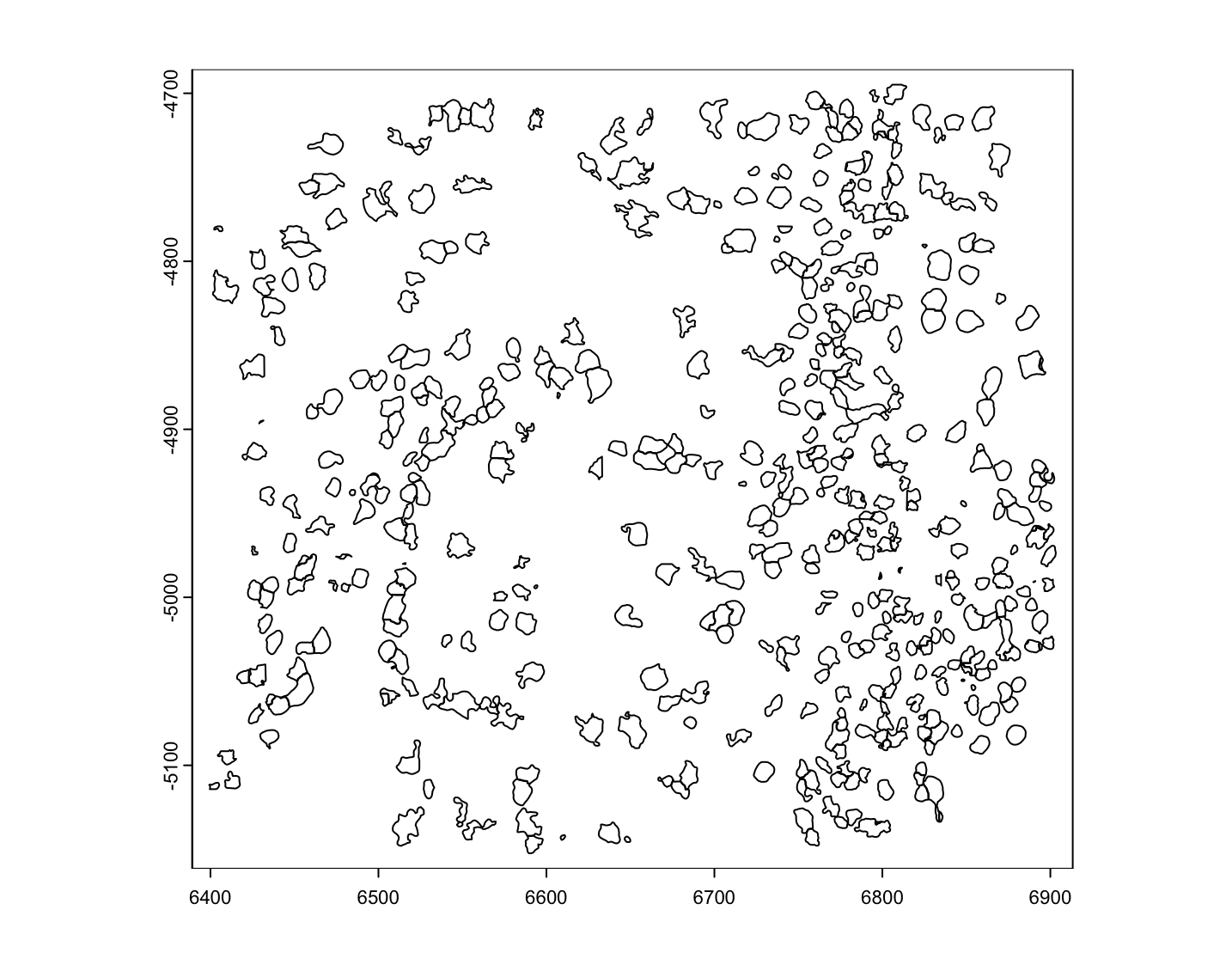
Points information can be read into GiottoSuite from any
data.frame-like object with points coordinates information
(x, y, feat_ID). For most surety, the matching columns in the input
data.frame should be named with the colnames x, y, and
feat_ID, however createGiottoPoints() will attempt to guess
which columns are which. Additional columns if provided, will be
included as attributes information in the giottoPoints
object.
See also ?GiottoClass::createGiottoPoints
For this example, the following data.table will be
used.
tx_dt <- data.table::fread(mini_viz_tx_path)
tx_dt[, global_y := -global_y] # flip values to match polys
# (this can also be done after `giottoPoints` creation using flip())
force(tx_dt)
global_x global_y gene global_z
<num> <num> <char> <int>
1: 6400.037 -4966.651 Mlc1 0
2: 6400.041 -4965.377 Gprc5b 0
3: 6400.078 -5081.453 Gfap 0
4: 6400.084 -5038.288 Gfap 0
5: 6400.172 -4816.516 Ednrb 0
---
80339: 6900.010 -4773.595 Adgra1 1
80340: 6900.023 -4772.980 Cspg5 1
80341: 6900.024 -5007.432 Adcyap1r1 1
80342: 6900.026 -4924.840 Slc17a7 1
80343: 6900.030 -4746.916 Cldn5 1
viz_gpoints <- createGiottoPoints(tx_dt)

force(viz_gpoints)
An object of class giottoPoints
feat_type : "rna"
Feature Information:
class : SpatVector
geometry : points
dimensions : 80343, 3 (geometries, attributes)
extent : 6400.037, 6900.032, -5149.983, -4699.979 (xmin, xmax, ymin, ymax)
coord. ref. :
names : feat_ID global_z feat_ID_uniq
type : <chr> <int> <int>
values : Mlc1 0 1
Gprc5b 0 2
Gfap 0 3
plot(viz_gpoints)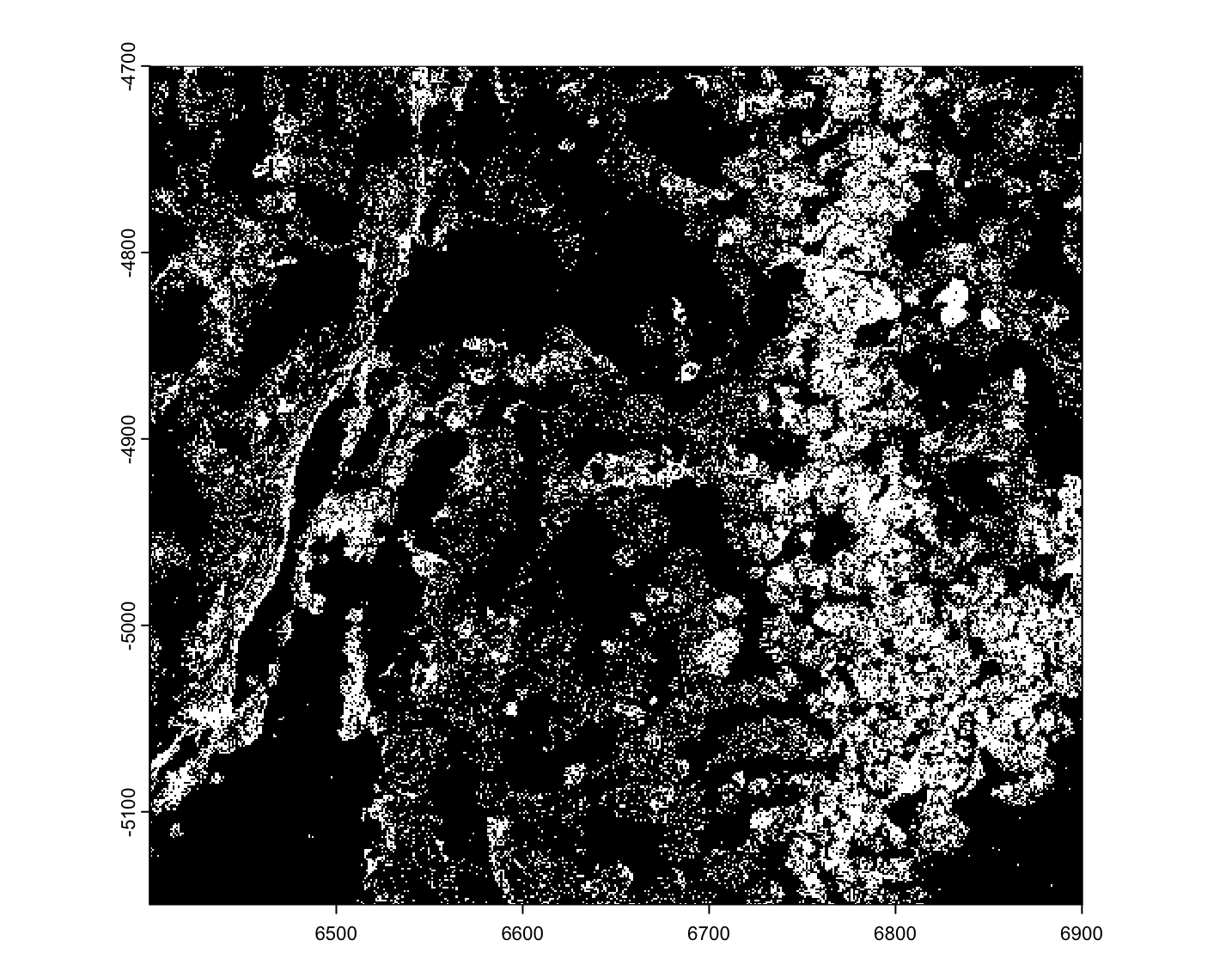
3 Checking spatial alignment
Care should always be taken when assembling a spatial dataset to make sure that the spatial information is spatially aligned. We can check this by plotting the subobjects. When the data is not properly aligned, the polygons will extract incorrect features or even find no values.
plot(viz_gpoints, raster = FALSE)
# raster = TRUE is default and faster, but does not work with additive plotting
plot(viz_gpoly, add = TRUE, border = "cyan", lwd = 0.7)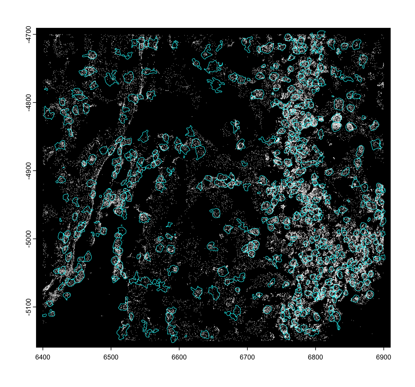
These plots can take a long time depending on how large the dataset
is. For very large dataset, it is a good idea to designate a smaller ROI
using ext() then plotting just that ROI.
# example plot with ROI. This is a good idea for large datasets.
ROI <- ext(c(6500, 6700, -5000, -4800)) # xmin, xmax, ymin, ymax
plot(viz_gpoints, raster = FALSE, ext = ROI)
# raster = TRUE is default and faster, but does not work with additive plotting
plot(viz_gpoly, add = TRUE, border = "cyan", lwd = 0.7, ext = ROI)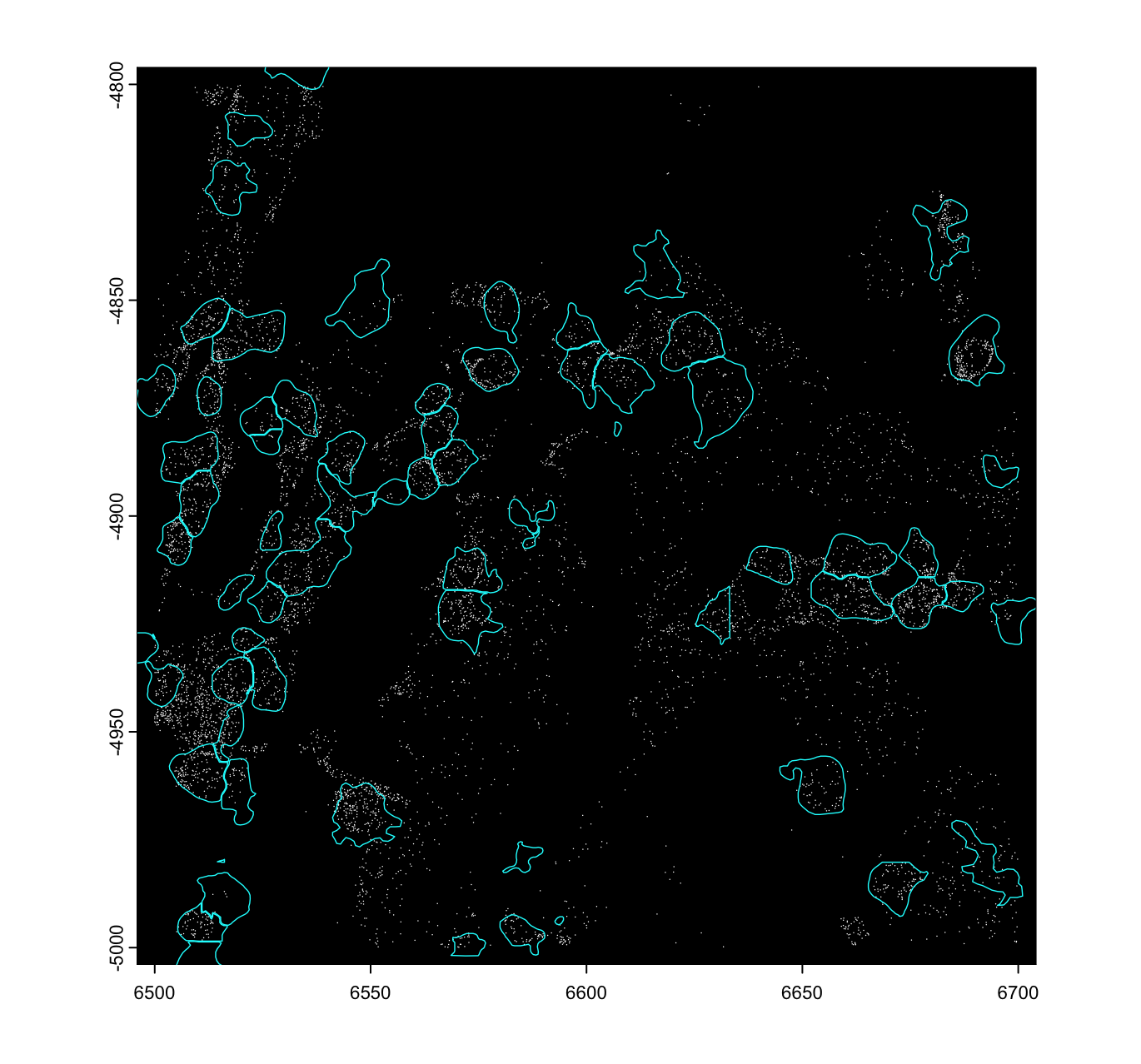
4 Creating the subcellular Giotto object
Datasets with raw spatial features and polygon information are
created using createGiottoObjectSubcellular().
mini_viz <- createGiottoObjectSubcellular(
  gpolygons = viz_gpoly,
  gpoints = viz_gpoints
)

force(mini_viz)
An object of class giotto
[SUBCELLULAR INFO]
polygons : cell
features : rna
[AGGREGATE INFO]
Use objHistory() to see steps and params used5 Spatially aggregate values
This operation tallies up the transcript detections under each of the polygon annotations and then converts that into a raw counts matrix.
# calculate centroids
mini_viz <- addSpatialCentroidLocations(mini_viz)
# create aggregated information
mini_viz <- calculateOverlap(mini_viz)
mini_viz <- overlapToMatrix(mini_viz)
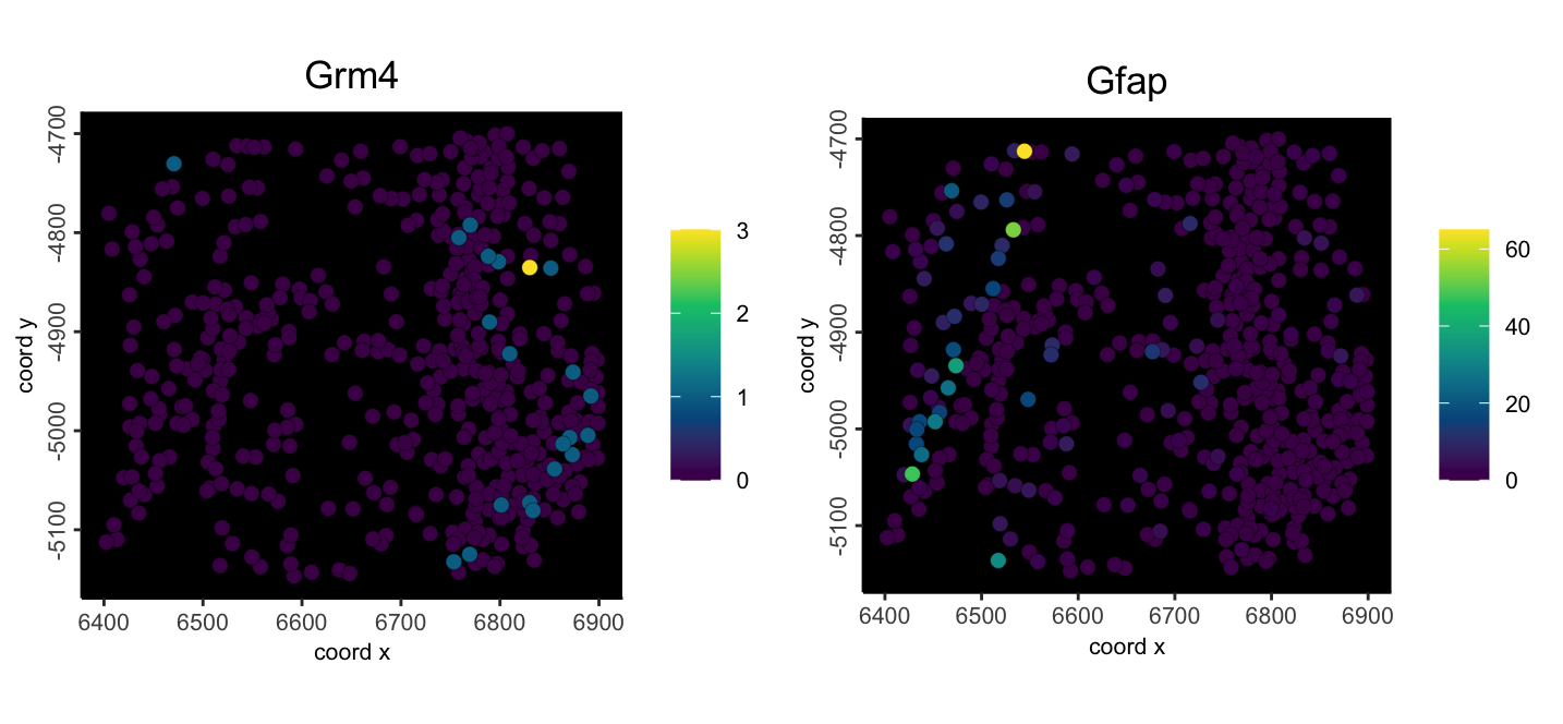
6 Example plot
spatFeatPlot2D(
  mini_viz,
  feats = c("Grm4", "Gfap"),
  expression_values = "raw",
  point_size = 2.5,
  gradient_style = "sequential",
  background_color = "black"
)
7 Session Info
R version 4.4.1 (2024-06-14)
Platform: aarch64-apple-darwin20
Running under: macOS 15.0.1

Matrix products: default
BLAS:   /System/Library/Frameworks/Accelerate.framework/Versions/A/Frameworks/vecLib.framework/Versions/A/libBLAS.dylib
LAPACK: /Library/Frameworks/R.framework/Versions/4.4-arm64/Resources/lib/libRlapack.dylib;  LAPACK version 3.12.0

locale:
[1] en_US.UTF-8/en_US.UTF-8/en_US.UTF-8/C/en_US.UTF-8/en_US.UTF-8

time zone: America/New_York
tzcode source: internal

attached base packages:
[1] stats     graphics  grDevices utils     datasets  methods   base

other attached packages:
[1] Giotto_4.1.5      GiottoClass_0.4.3

loaded via a namespace (and not attached):
 [1] tidyselect_1.2.1            viridisLite_0.4.2           farver_2.1.2
 [4] dplyr_1.1.4                 R.utils_2.12.3              GiottoVisuals_0.2.7
 [7] fastmap_1.2.0               SingleCellExperiment_1.26.0 lazyeval_0.2.2
[10] digest_0.6.37               lifecycle_1.0.4             terra_1.7-78
[13] magrittr_2.0.3              compiler_4.4.1              rlang_1.1.4
[16] tools_4.4.1                 igraph_2.1.1                utf8_1.2.4
[19] yaml_2.3.10                 data.table_1.16.2           knitr_1.48
[22] labeling_0.4.3              S4Arrays_1.4.0              htmlwidgets_1.6.4
[25] reticulate_1.39.0           DelayedArray_0.30.0         xml2_1.3.6
[28] abind_1.4-8                 withr_3.0.1                 purrr_1.0.2
[31] R.oo_1.26.0                 BiocGenerics_0.50.0         grid_4.4.1
[34] stats4_4.4.1                fansi_1.0.6                 colorspace_2.1-1
[37] progressr_0.14.0            ggplot2_3.5.1               scales_1.3.0
[40] gtools_3.9.5                SummarizedExperiment_1.34.0 cli_3.6.3
[43] rmarkdown_2.28              crayon_1.5.3                generics_0.1.3
[46] rstudioapi_0.16.0           httr_1.4.7                  rjson_0.2.21
[49] stringr_1.5.1               zlibbioc_1.50.0             parallel_4.4.1
[52] XVector_0.44.0              matrixStats_1.4.1           vctrs_0.6.5
[55] Matrix_1.7-0                jsonlite_1.8.9              IRanges_2.38.0
[58] S4Vectors_0.42.0            ggrepel_0.9.6               scattermore_1.2
[61] systemfonts_1.1.0           magick_2.8.5                GiottoUtils_0.2.1
[64] plotly_4.10.4               tidyr_1.3.1                 glue_1.8.0
[67] codetools_0.2-20            cowplot_1.1.3               stringi_1.8.4
[70] gtable_0.3.5                GenomeInfoDb_1.40.0         GenomicRanges_1.56.0
[73] UCSC.utils_1.0.0            munsell_0.5.1               tibble_3.2.1
[76] pillar_1.9.0                htmltools_0.5.8.1           GenomeInfoDbData_1.2.12
[79] R6_2.5.1                    evaluate_1.0.0              kableExtra_1.4.0
[82] lattice_0.22-6              Biobase_2.64.0              highr_0.11
[85] R.methodsS3_1.8.2           png_0.1-8                   backports_1.5.0
[88] SpatialExperiment_1.14.0    Rcpp_1.0.13                 svglite_2.1.3
[91] SparseArray_1.4.1           checkmate_2.3.2             colorRamp2_0.1.0
[94] xfun_0.47                   MatrixGenerics_1.16.0       pkgconfig_2.0.3