Giotto Object Creation - Intensity Image Data
Source:vignettes/obj_create_img.Rmd
obj_create_img.Rmd1 Setup Giotto and download data to use
# Ensure Giotto Suite is installed.
if(!"Giotto" %in% installed.packages()) {
  pak::pkg_install("drieslab/Giotto")
}
# Ensure the Python environment for Giotto has been installed.
genv_exists <- Giotto::checkGiottoEnvironment()
if(!genv_exists){
  # The following command need only be run once to install the Giotto environment.
  Giotto::installGiottoEnvironment()
}

library(Giotto)
The IMC data to run this tutorial can be found in the
imcdatasets package. We will be using one of the smaller
example datasets. These IMC outputs provide multilayer images in the
format of cytomapper CytoImageList collections of
EBImage Image objects, which can be easily coerced
to simple matrices.
The package exactextractr is also used due to its speed with image data extractions.
# Ensure imcdatasets and exactextractr are installed.
if(!"imcdatasets" %in% installed.packages()) {
    # this should also ensure cytomapper is installed
  pak::pkg_install("imcdatasets")
}
if(!"exactextractr" %in% installed.packages()) {
  pak::pkg_install("exactextractr")
}

# load dataset
imc_masks <- imcdatasets::IMMUcan_2022_CancerExample("masks")
imc_imgs <- imcdatasets::IMMUcan_2022_CancerExample("images")

# coerce to matrix
mask_mat <- imc_masks$Patient1_001[]
img_mat <- lapply(
    seq_len(dim(imc_imgs$Patient1_001)[3]),
    function(lyr) imc_imgs$Patient1_001[][,,lyr]
)
channels <- cytomapper::channelNames(imc_imgs)
2 Read data into Giotto Suite
Polygons can be read into Giotto Suite in multiple ways.
When using createGiottoPolygon():
- If a
characterinput is provided, it is assumed to be a filepath to a .GeoJSON or mask image file. Which it is is determined based on file extension. - If a
data.frameis provided, then it is expected to be adata.framewith vertex X, Y, and poly_ID information. The columns can be guessed, but naming them specificallyx,y, andpoly_IDwill ensure that the correct ones are picked.
You can also be more explicit about the type of input provided by
calling any of the following directly, instead of having
createGiottoPolygon() guess.
See also ?GiottoClass::createGiottoPolygon
For this example we have a matrix input, which is not
yet one of the datatypes automatically understood by
createGiottoPolygon(), so we specifically pass it to
createGiottoPolygonsFromMask().
# create the mask polys
mask_poly <- createGiottoPolygonsFromMask(mask_mat,
    shift_vertical_step = -1,
    flip_vertical = FALSE,
    flip_horizontal = FALSE,
    shift_horizontal_step = FALSE,
    remove_background_polygon = TRUE
    # remove polygons that cover most of the spatial extent of the dataset
    # (these are usually artefact background polys)
)
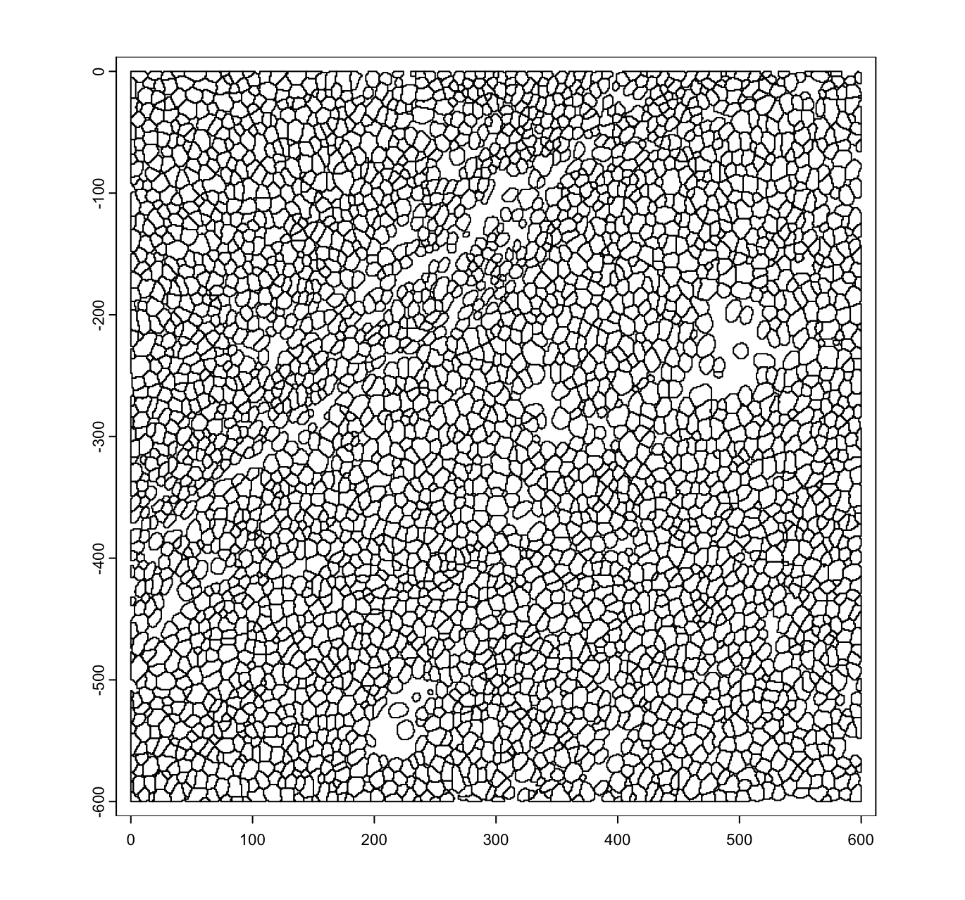
force(mask_poly)
An object of class giottoPolygon
spat_unit : "cell"
Spatial Information:
class : SpatVector
geometry : polygons
dimensions : 3567, 1 (geometries, attributes)
extent : 0, 600, -600, 0 (xmin, xmax, ymin, ymax)
coord. ref. :
names : poly_ID
type : <chr>
values : cell_1
cell_2
cell_3
centroids : NULL
overlaps : NULL
plot(mask_poly)
# load the image matrices in as a list of `giottoLargeImages`
imglist <- lapply(seq_along(img_mat), function(img_i) {
    createGiottoLargeImage(img_mat[[img_i]], name = channels[[img_i]])
})
names(imglist) <- channels
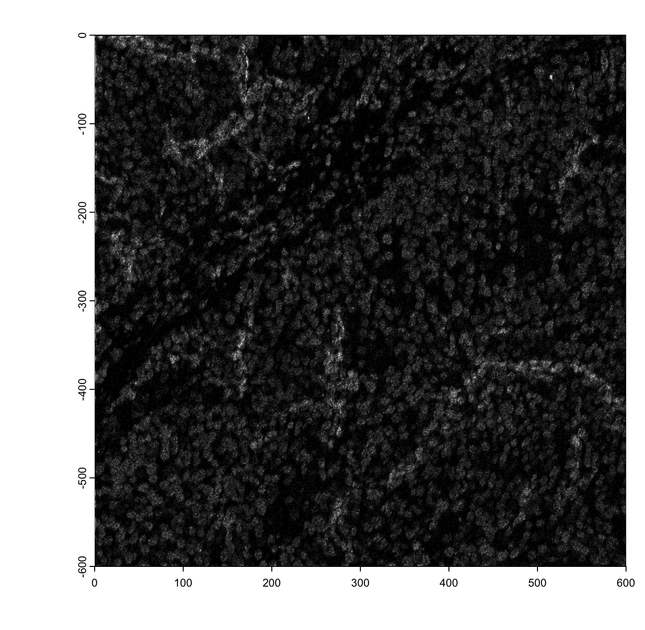
force(imglist[["H3"]])
An object of class giottoLargeImage : "H3"
Image extent : 0, 600, -600, 0 (xmin, xmax, ymin, ymax)
Original image extent : 0, 600, -600, 0 (xmin, xmax, ymin, ymax)
Scale factor : 1, 1 (x, y)
Resolution : 1, 1 (x, y)
Layers : 1
Estimated max intensity : 60.95492
Estimated min intensity : 0
Values : floating point
File path : ''
plot(imglist[["H3"]], max_intensity = 30)
4 Creating the giotto object
imc <- createGiottoObjectSubcellular(
    gpolygons = mask_poly,
    images = imglist
)
force(imc)
An object of class giotto
>Active spat_unit: cell
dimensions : NA, 3567 (features, cells)
[SUBCELLULAR INFO]
polygons : cell
[AGGREGATE INFO]
attached images ------------------
images : 40 items...
Use objHistory() to see steps and params usedNote that we already have a cells count because of the polygons
information, but the number of features is still NA. This
field will be populated once we aggregate the image intensity values to
be used as features.
5 Spatially aggregate values
This operation finds the pixels overlapped by the cell annotations. For each cell, the intensities of all pixels covered will be taken and summed (by default) to generate a raw feature matrix.
# calculate centroids
imc <- addSpatialCentroidLocations(imc)
# create aggregated information
imc <- calculateOverlap(imc, image_names = channels, name_overlap = "protein")
imc <- overlapToMatrix(imc, type = "intensity", feat_info = "protein")
force(imc)
An object of class giotto
>Active spat_unit: cell
>Active feat_type: protein
dimensions : 40, 3567 (features, cells)
[SUBCELLULAR INFO]
polygons : cell
[AGGREGATE INFO]
expression -----------------------
[cell][protein] raw
spatial locations ----------------
[cell] raw
attached images ------------------
images : 40 items...
Use objHistory() to see steps and params usedThis is now a giotto object with 3567 cells and 40
features, one feature for each of the input intensity images.
6 Example plot
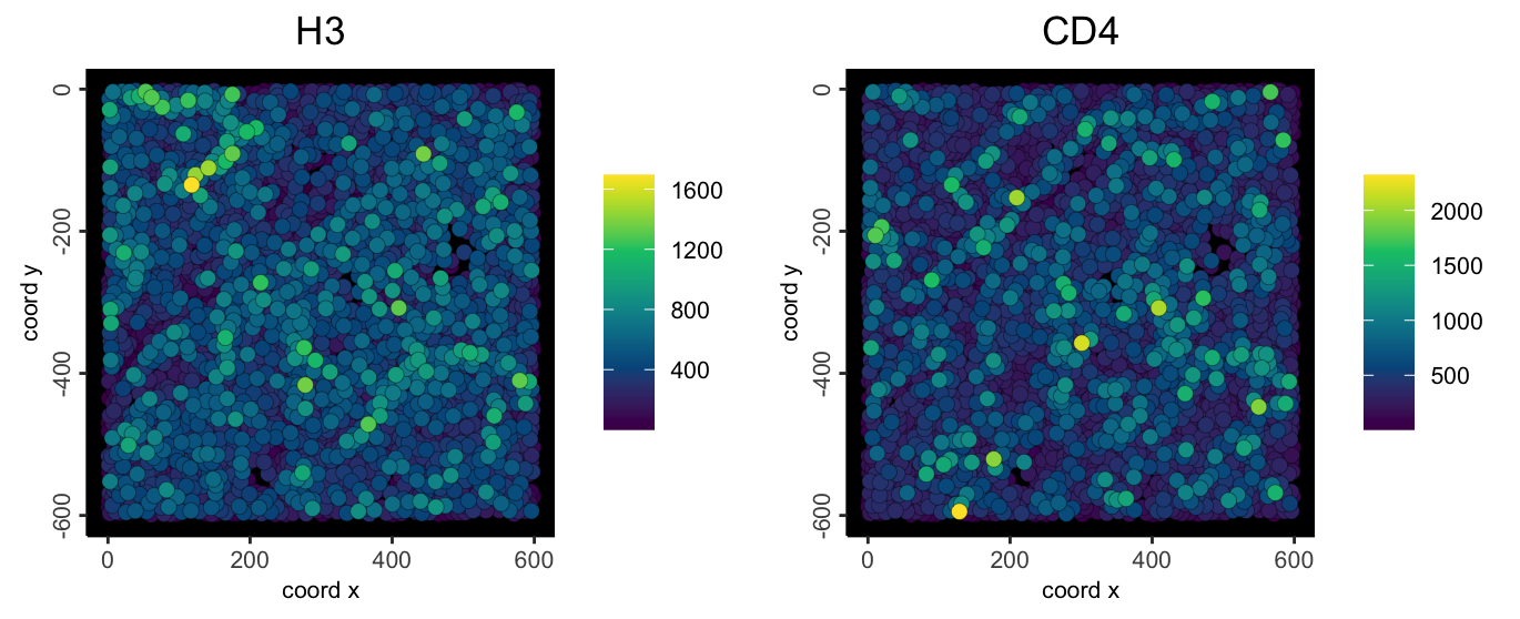
spatFeatPlot2D(
  imc,
  feats = c("H3", "CD4"),
  expression_values = "raw",
  point_size = 2.5,
  gradient_style = "sequential",
  background_color = "black"
)
Note: If you notice a single extremely bright center spot, then there was likely a background polygon that was not removed.
7 Session Info
R version 4.4.1 (2024-06-14)
Platform: aarch64-apple-darwin20
Running under: macOS 15.0.1

Matrix products: default
BLAS:   /System/Library/Frameworks/Accelerate.framework/Versions/A/Frameworks/vecLib.framework/Versions/A/libBLAS.dylib
LAPACK: /Library/Frameworks/R.framework/Versions/4.4-arm64/Resources/lib/libRlapack.dylib;  LAPACK version 3.12.0

locale:
[1] en_US.UTF-8/en_US.UTF-8/en_US.UTF-8/C/en_US.UTF-8/en_US.UTF-8

time zone: America/New_York
tzcode source: internal

attached base packages:
[1] stats4    stats     graphics  grDevices utils     datasets  methods   base

other attached packages:
 [1] imcdatasets_1.12.0          cytomapper_1.16.0           EBImage_4.46.0
 [4] SpatialExperiment_1.14.0    SingleCellExperiment_1.26.0 SummarizedExperiment_1.34.0
 [7] Biobase_2.64.0              GenomicRanges_1.56.0        GenomeInfoDb_1.40.0
[10] IRanges_2.38.0              S4Vectors_0.42.0            BiocGenerics_0.50.0
[13] MatrixGenerics_1.16.0       matrixStats_1.4.1           Giotto_4.1.5
[16] GiottoClass_0.4.3

loaded via a namespace (and not attached):
  [1] later_1.3.2             bitops_1.0-8            filelock_1.0.3
  [4] tibble_3.2.1            R.oo_1.26.0             svgPanZoom_0.3.4
  [7] lifecycle_1.0.4         sf_1.0-16               lattice_0.22-6
 [10] exactextractr_0.10.0    backports_1.5.0         magrittr_2.0.3
 [13] plotly_4.10.4           rmarkdown_2.28          yaml_2.3.10
 [16] httpuv_1.6.15           sp_2.1-4                reticulate_1.39.0
 [19] cowplot_1.1.3           DBI_1.2.3               RColorBrewer_1.1-3
 [22] abind_1.4-8             zlibbioc_1.50.0         purrr_1.0.2
 [25] R.utils_2.12.3          RCurl_1.98-1.16         rappdirs_0.3.3
 [28] GenomeInfoDbData_1.2.12 ggrepel_0.9.6           terra_1.7-78
 [31] units_0.8-5             svglite_2.1.3           colorRamp2_0.1.0
 [34] codetools_0.2-20        DelayedArray_0.30.0     xml2_1.3.6
 [37] tidyselect_1.2.1        raster_3.6-26           UCSC.utils_1.0.0
 [40] farver_2.1.2            viridis_0.6.5           BiocFileCache_2.12.0
 [43] jsonlite_1.8.9          e1071_1.7-14            progressr_0.14.0
 [46] systemfonts_1.1.0       tools_4.4.1             Rcpp_1.0.13
 [49] glue_1.8.0              gridExtra_2.3           SparseArray_1.4.1
 [52] xfun_0.47               dplyr_1.1.4             HDF5Array_1.32.0
 [55] shinydashboard_0.7.2    withr_3.0.1             BiocManager_1.30.23
 [58] fastmap_1.2.0           rhdf5filters_1.16.0     fansi_1.0.6
 [61] digest_0.6.37           R6_2.5.1                mime_0.12
 [64] colorspace_2.1-1        scattermore_1.2         gtools_3.9.5
 [67] jpeg_0.1-10             RSQLite_2.3.6           R.methodsS3_1.8.2
 [70] utf8_1.2.4              tidyr_1.3.1             generics_0.1.3
 [73] data.table_1.16.2       class_7.3-22            httr_1.4.7
 [76] htmlwidgets_1.6.4       S4Arrays_1.4.0          pkgconfig_2.0.3
 [79] gtable_0.3.5            blob_1.2.4              GiottoVisuals_0.2.7
 [82] XVector_0.44.0          htmltools_0.5.8.1       fftwtools_0.9-11
 [85] scales_1.3.0            kableExtra_1.4.0        GiottoUtils_0.2.1
 [88] png_0.1-8               knitr_1.48              rstudioapi_0.16.0
 [91] rjson_0.2.21            checkmate_2.3.2         curl_5.2.3
 [94] proxy_0.4-27            cachem_1.1.0            rhdf5_2.48.0
 [97] stringr_1.5.1           KernSmooth_2.23-24      BiocVersion_3.19.1
[100] parallel_4.4.1          vipor_0.4.7             AnnotationDbi_1.66.0
[103] pillar_1.9.0            grid_4.4.1              vctrs_0.6.5
[106] promises_1.3.0          dbplyr_2.5.0            xtable_1.8-4
[109] beeswarm_0.4.0          evaluate_1.0.0          magick_2.8.5
[112] cli_3.6.3               locfit_1.5-9.9          compiler_4.4.1
[115] rlang_1.1.4             crayon_1.5.3            labeling_0.4.3
[118] classInt_0.4-10         ggbeeswarm_0.7.2        stringi_1.8.4
[121] viridisLite_0.4.2       BiocParallel_1.38.0     nnls_1.5
[124] munsell_0.5.1           Biostrings_2.72.0       lazyeval_0.2.2
[127] tiff_0.1-12             Matrix_1.7-0            ExperimentHub_2.12.0
[130] bit64_4.5.2             ggplot2_3.5.1           Rhdf5lib_1.26.0
[133] KEGGREST_1.44.0         shiny_1.9.1             highr_0.11
[136] AnnotationHub_3.12.0    igraph_2.1.1            memoise_2.0.1
[139] bit_4.5.0 